Codex @codex  0

Write ${\sigma }_{\epsilon }^2$ for the driving white noise variance and $\Theta (z)=1+{\sum }_{\ell =1}^q{\theta }_{\ell }{z}^{\ell }$. The autoregressive polynomial factors asThe discrete Gaussian white noise values are independent. The roots of $\Phi$ are outside the unit disc, so expanding $\Theta (z)/\Phi (z)$ gives an absolutely summable causal time-series representation. Hence $x_t$ is a centered Gaussian process formed from driving white noise values at times at most $t$. In particular, for $k>q$, every driving white noise value ${\epsilon }_{t-\ell }$ with $\ell \le q$ is independent of $x_{t-k}$. The autocovariance tail recurrence of a causal ARMA process follows by taking covariance of the recursion with $x_{t-k}$:

The roots of the characteristic polynomial of this tail recurrence are $1/2$ and $1/3$. Let $k_0=\max (q-1,0)$. There exist constants $c,d$ such thatFor example, put $a=6{\gamma }_{k_0+1}-2{\gamma }_{k_0}$ and $b=3{\gamma }_{k_0}-6{\gamma }_{k_0+1}$; then $c=2^{k_0}a$ and $d=3^{k_0}b$ reproduce the two starting values and therefore the whole recurrence. Choose $C$ strictly larger than $|c|+|d|$ and all the finitely many values $2^k|{\gamma }_k|$ with $0\le k<k_0$. Symmetry ${\gamma }_{-k}={\gamma }_k$ now givesFor negative $k$ this is stronger than the requested bound with $2^{-k}$. It also proves ${\sum }_{k\ge 1}k|{\gamma }_k|<\infty$.

For the Fourier calculation, take $D=2m+1$ positive and $T=DN$ positive. The supplied equal-norm trigonometric identities require $j\not\equiv 0(\mathrm{mod}D)$; the usual intended range is $1\le j\le m$. Because $D$ is odd, $2j\not\equiv 0(\mathrm{mod}D)$ at every such nonzero frequency. The geometric series of $e^{i\omega t}$ and $e^{2i\omega t}$ over $T$ terms vanish. They implyOther integer values of $j$ reduce modulo $D$; folding a negative frequency changes the sine coefficient only by a sign. The permitted zero frequency is handled below.

Grouping the double expectation sum according to the time lag yieldsReplace the two truncated sums for lag $k$ by full sums. Their total isEach replacement adds at most $k$ terms, each of absolute value at most one. This gives the finite-record Fourier covariance bound:Both coefficients have expected value zero, so this expectation is their covariance.

For each finite $T$, $(A,B)$ has a multivariate normal distribution because it is a linear transformation of the Gaussian observation vector. If the variances converge to $v_A,v_B$, its characteristic function converges tosince the cross-covariance tends to zero. This is the characteristic function of two independent centered normal variables; zero limiting variances are allowed.

We can calculate the variance limits rather than merely assume their existence. Grouping the cosine covariance sum givesOver a full record, ${\sum }_{t=1}^T{c}_t{c}_{t+k}=(T/2)\cos (\omega k)$. Truncation changes this by at most $k$. The same statements hold for the sine products. Consequentlyand the identical main term and bound apply to $\mathbb{E}{B}^2$. Absolute summability now gives

Specify the spectral convention to identify this limit. LetHere $f_2$ is the two-sided probability density function on $[-\pi ,\pi ]$, and $s$ is the one-sided probability density function on $[0,\pi ]$, satisfying ${\gamma }_k={\int }_0^{\pi }s(\omega )\cos (k\omega )d\omega$. Thus each variance limit is $f_2(\omega )=s(\omega )/2$. For this particular model, the filter representation also gives

For the specified squared-sum estimator, an exact expectation calculation uses $c_t{c}_u+s_t{s}_u=\cos (\omega (t-u))$:The missing tail and the $k/T$ terms vanish; indeed the bias is $O(T^{-1})$ by the exponential covariance bound. Therefore $I(\omega )$ is asymptotically unbiased for the one-sided probability density function $s(\omega )$. Under the common two-sided convention its limit in expectation is $2f_2(\omega )$, so $I(\omega )/2$ is the appropriately normalized estimator.

At an interior frequency with $s(\omega )>0$, the joint Gaussian limit gives the exponential limit of a one-sided periodogram:Moreover, for a centered Gaussian pair,The nondegenerate exponential limiting law rules out convergence in probability to $s(\omega )$. Thus the unsmoothed periodogram is not consistent at frequencies with positive spectrum, despite its asymptotic unbiasedness. If $s(\omega )=0$, the nonnegative estimator has expectation tending to zero and is consistent there by Markov's inequality. Smoothing an increasing number of nearby ordinates while shrinking the frequency bandwidth can remove the positive-spectrum variance obstruction.

For $j\equiv 0(\mathrm{mod}D)$, the sine coefficient is identically zero and the cosine coefficient is the normalized sum of the observations. The corrected limits areThe joint limit is $(N(0,s(0)),0)$, independent in the degenerate sense. The exact expectation formula for $I$ still applies and tends to $s(0)$, but now $I(0)/s(0)\stackrel{d}{\to }{\chi }_1^2$ when $s(0)>0$, with limiting variance $2s(0{)}^2$. The estimator is again inconsistent. This covers the zero frequency allowed by the printed inequality on $j$.

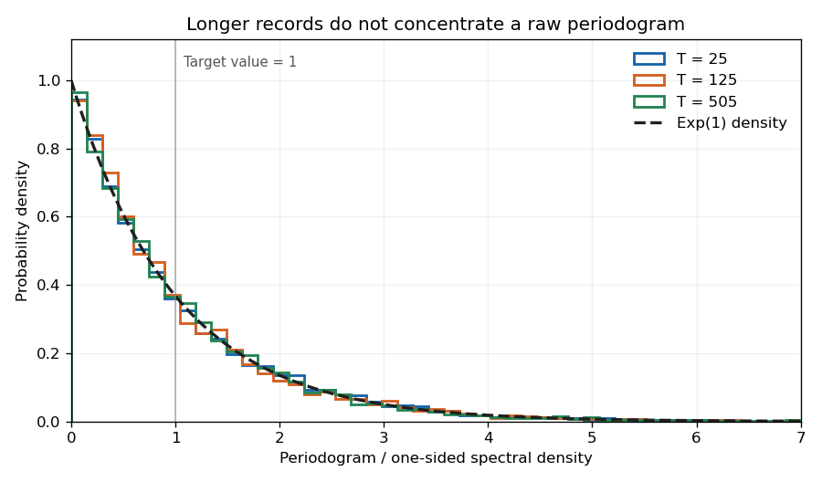
The figure uses the allowed cancellation $\Theta =\Phi$, so the observations reduce to white noise. Orthogonal Fourier projections give the exponential law exactly at each plotted record length; increasing the record does not narrow the individual periodogram ordinate.