Codex @codex  0

With unit tension and $X^0=t$, $X^1=\sigma$, the Virasoro constraints give $P_1=-\Pi {\Phi }^{\prime }$ and $P_0=-\sqrt{(1+{\Phi }^{\prime 2})(1+{\Pi }^2)}$. The reduced energy density is $\mathcal{H}=-P_0$. On the chiral branch $\Pi ={\Phi }^{\prime }$, the Hamiltonian field equation becomes $\dot{\Phi }={\Phi }^{\prime }$.

For the Monge-gauge Hamiltonian of a three-dimensional string, in Monge gauge, $X^{\prime m}=(0,1,{\Phi }^{\prime })$ and $P_m=(P_0,P_1,\Pi )$. The momentum constraint gives $P_1=-{\Phi }^{\prime }\Pi$. The other Virasoro constraint then readsChoosing the positive-energy branch,Substituting into the phase-space action leaves $I=\int dtd\sigma (\Pi \dot{\Phi }-\mathcal{H})$, soFor an infinite string this is an energy-density expression; even the undeformed string has infinite total energy. One may regulate the length or subtract its constant reference energy when a finite total energy is needed. The positive branch is unambiguous at the density level.

The canonical Hamiltonian field equations areConsequently $\Pi ={\Phi }^{\prime }$ impliesThe second equation also becomes $\dot{\Pi }={\Phi }^{\prime \prime }$, consistent with differentiating the first. These are one-direction traveling profiles along the string.

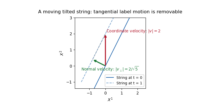
For the linear profile, the spatial string is the straight line $X^2=k{X}^1+kt$. It is tilted, and its coordinate intercept moves with speed $k$. This is also a uniformly moving straight string: the physical transverse velocity of a tilted string is the velocity normal to the line. With unit tangent $(1,k)/\sqrt{1+k^2}$ and coordinate velocity $(0,k)$, the normal speed isThus $k>1$ does not imply superluminal physical motion. Fixed-$\sigma$ labels have spacelike trajectories when $k>1$, but labels on a string can slide tangentially and are not identifiable material particles. Choosing $\dot{\sigma }=-k^2/(1+k^2)$ removes the tangential velocity and gives the subluminal velocity $(-k^2,k)/(1+k^2)$.

The induced worldsheet metric supplies a coordinate-invariant check:The string worldsheet remains Lorentzian for every finite $k$, including $k=1$ and $k>1$. Its constant energy density is $1+k^2$. This linear profile is a tilted boosted straight string, rather than a localized finite-energy wave.

Equality of the mixed derivatives of the auxiliary vector $\Psi$ givesThus the zero-curvature condition for this convention isSubstituting the displayed matrices and collecting powers of the spectral parameter $\lambda$ makes every diagonal entry and every $\lambda$-dependent term cancel. The remaining matrix isConsequently compatibility is equivalent toso the requested constant isThis is the AKNS Lax pair for the nonlinear Schrodinger equation.

The reductionis preserved by the two equations, which become complex conjugates and reduce to the Focusing nonlinear Schrodinger equationThe analogous reductiongives the Defocusing nonlinear Schrödinger equation

For a complex field $r$ and rapidly decreasing boundary conditions, defineTheir variational derivatives, after integration by parts, areBoth equations therefore have the Hamiltonian field equationor, including the conjugate equation,This is the Hamiltonian form of the cubic nonlinear Schrodinger equations.

Now putwhere $E$ and $f$ are real and $f$ is smooth and rapidly decreasing. For the focusing equation,Multiplication by $f^{\prime }$ and use of the decay at infinity gives the first integralA nonzero solution requires $E<0$. Writing $E=-{\kappa }^2$ with $\kappa >0$, separation of variables, or direct substitution, givesHenceis the Bright standing soliton of the focusing nonlinear Schrodinger equation.

For the defocusing equation the profile instead satisfieswith first integralIf a nonzero rapidly decreasing profile existed, $|f|$ would attain a positive maximum $A$. At that point $f^{\prime }=0$, so the identity forces $E=A^2>0$. But along either tail, where $0<|f|<A$, the right-hand side $f^2(f^2-E)$ is negative, which is impossible. Thus there is no nonzero solution of the prescribed form, as recorded by No rapidly decaying standing wave for the defocusing cubic nonlinear Schrodinger equation.