For a nonrelativistic point mass of fixed mass , measured in an inertial frame, its momentum isMomentum is a vector pointing along the velocity, with International System of Units unit . Doubling either mass or velocity doubles momentum. In one dimension, a chosen positive direction makes a signed quantity: a body moving right at has ; moving left at the same speed gives . [ref]
For a collection, total momentum is the vector sum . Two equal masses moving with opposite velocities can have zero total momentum while both have positive kinetic energy. Direction is therefore essential when using momentum conservation; adding speeds instead of signed velocities gives the wrong balance.
Newton's second law connects the net force on one fixed-mass point mass to its momentum through . Integrating that change gives impulse. Here denotes mechanical momentum; when canonical momentum differs from mass times velocity, the distinction in mechanical momentum below applies. The nonrelativistic formula also has a limited regime: special relativity is needed at speeds comparable with the speed of light.
For a massive particle, its spatial momentum in an inertial frame is , with m its invariant rest mass and the Lorentz factor. Together with its relativistic energy it forms the four-momentum. In a magnetic quadrupole's paraxial approximation, replacing by the longitudinal momentum extends the transverse focusing scale to relativistic beams.
For a charged particle minimally coupled to a magnetic vector potential, the mechanical momentum is , with the canonical momentum. It is the mass times velocity in nonrelativistic mechanics.
Momentum conservation states that total momentum stays constant when the net force exerted from outside the chosen collection is zero. Use a closed collection, meaning the same fixed-mass point masses are followed throughout, and an inertial frame. ThenTo see why, sum Newton's second law over the members. If is the force on member from member , Newton's third law assumes . Each pair cancels in the total:The internal forces act on different bodies and can change their individual momenta; their contributions cancel only in the collection's sum. An isolated system has no external interaction, but balanced external forces also suffice for momentum conservation. A closed system merely excluding matter exchange need not have conserved momentum. [ref]
https://openstax.org/books/university-physics-volume-1/pages/9-3-conservation-of-linear-momentum. OpenStax University Physics Volume 1, section 9.3: Conservation of Linear Momentum
The usefulness is that the detailed internal forces during a collision need not be known. Both an elastic collision and a perfectly inelastic collision obey the same isolated momentum balance; kinetic energy conservation is an additional condition for the elastic collision. If the external impulse is small but nonzero, the total momentum change is correspondingly small. For a variable-mass system exchanging matter, the entering or leaving momentum must also be included.
In a translation-invariant field theory, integrating over the spacetime zero mode enforces momentum conservation at interactions and scattering amplitudes.
If a mass m moving at u splits into equal fragments at velocities , conservation of momentum fixes their centre-of-mass velocity. Their kinetic energy increases by , independent of u. Thus an internal release energy Q gives . A front fragment must exceed a leading target's speed to close a pre-existing separation; merely matching speed does not intercept it. This kinematic result does not specify subsequent capture or braking.
For downward pre-ejection speed , total mass , payload mass , and downward payload speed in the original inertial frame, the remaining body's upward speed is . When the numerator nearly cancels, distinguishing total initial mass from final body mass is essential.
Recoil is the motion acquired by a body when it exchanges momentum with an emitted, absorbed or scattered particle. For isolated emission from a body initially at rest, momentum conservation makes the remaining body acquire the opposite momentum. If its final mass is and the recoil is nonrelativistic, its kinetic energy is . A photon of energy has momentum magnitude , so . The transition energy is shared between the photon and the recoiling body; nuclear recoil is an important example.
The ideal rocket equation gives the change in signed velocity produced by ejecting rocket propellant. Assume one-dimensional Newtonian mechanics in an inertial frame, no external force, and a fixed positive rocket exhaust speed directed rearward relative to the instantaneous rocket. The rocket's instantaneous mass includes its remaining rocket propellant; burning it gives . For initial and final masses ,Here is the natural logarithm, and its argument is the rocket mass ratio. This is the constant-rocket exhaust speed, zero-pressure-correction version of the ideal rocket equation. [ref]
For a toy rocket with , and rocket dry mass after all rocket propellant is spent, the rocket mass ratio is andBurning from to gains . Burning from to gains exactly the same velocity increment, using only of rocket propellant instead of . Both burns halve the remaining mass. The second burn accelerates a lighter rocket; equal fractional mass losses give equal velocity gains.
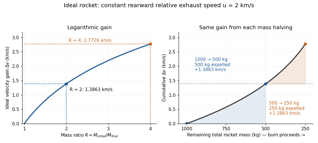
The natural logarithm makes the rocket equation both useful and revealing: multiplying successive rocket mass ratios adds their velocity gains. Conversely, the required rocket mass ratio is the exponential function . Each extra of ideal velocity gain doubles the required initial mass for fixed final mass. This explains why a larger rocket exhaust speed is valuable and why carrying ever more rocket propellant has diminishing returns. Changing the burn duration alone does not change this ideal endpoint result.
For a short proof outline, follow the rocket together with a tiny parcel about to be expelled. Before ejection, their total momentum is . After ejection, the remaining rocket has mass and velocity , while the parcel has positive mass and, to first order, inertial velocity . Momentum conservation givesDiscarding the second-order product gives ; taking the integral gives . Evaluating the integral yields the natural logarithm above. This is a variable-mass system calculation: the rocket alone is not a closed system, and its momentum changes as the expelled material carries away momentum. The fixed collection consisting of the rocket and all its expelled material has conserved total momentum when external forces vanish.
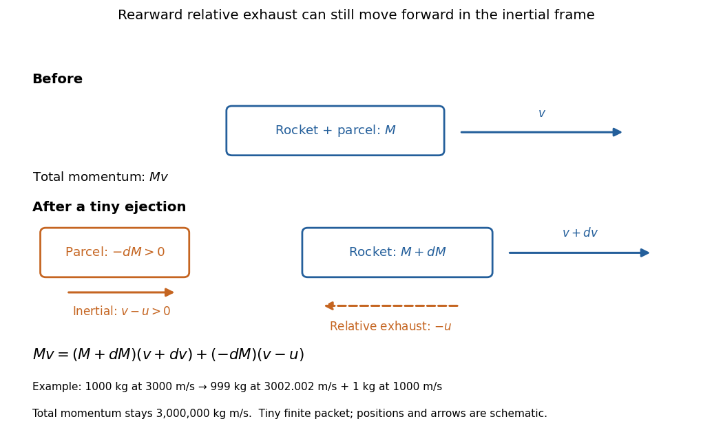
Momentum balance for a tiny expelled parcel: rearward relative exhaust can still move forward in the inertial frame
. Details. Fixed rocket exhaust speed means fixed relative speed at release, not fixed inertial velocity. As the rocket's velocity changes, newly emitted material has changing inertial velocity ; previously released parcels coast at their own release velocities in this ideal model. If , the exhaust even moves forward in the inertial frame, although it is emitted rearward relative to the rocket. No surrounding medium is needed for this exchange of momentum.
Real flight adds gravity, drag force and possibly a pressure correction to rocket thrust. A varying rocket thrust due solely to a changing mass loss rate still gives the same ideal rocket equation if is constant; it changes the acceleration and burn duration. A changing rocket exhaust speed instead requires , and external forces require their own contribution to the velocity change. The existing constant mass-loss propulsion with quadratic drag and constant-burn rocket with ground friction illustrate such additional forces; the forward-exhaust rocket equation reverses the ejection direction and therefore the sign of the recoil.
Two initially stationary rockets exchange a fuel load : A ejects it with constant rearward relative speed and B captures all of it. A has final velocity . Since final momentum is zero, . No elastic-capture assumption is needed. With negligible flight time, transferred mass gives the same balance with instantaneous masses and ; their opposite speeds are equal when those masses agree. Final complete collection is a condition on the model, not a guarantee that every ballistic exhaust trajectory intercepts B.
For exhaust moving freely from a rocket A toward a collector B behind it along a common axis, the exhaust must overtake B in the rearward direction. At negligible separation and flight time this gives the displayed condition. In the ideal simultaneous-collection solution, write , and , . The criterion becomes . A formal endpoint obtained by assuming all fuel is collected need not satisfy this interception test throughout a large burn.
A rocket discards exhausted stages, reducing the mass accelerated by later burns. Apply the rocket equation separately to each burn and add the signed velocity increments. Ideal jettison with no relative impulse leaves velocity continuous; it changes the mass ratio available to subsequent burns. Dry-stage mass must not be counted as propellant expelled at the rocket exhaust speed.
With downward speed , downward relative exhaust speed and mass , the ideal vertical equation is . Integration gives . Height follows from ; its touchdown condition must be imposed together with the final fuel fraction.
The rocket exhaust speed is the magnitude of the emitted material's velocity relative to the instantaneous rocket. In the ideal rearward-ejection convention of the rocket equation, a rocket with inertial velocity emits material with inertial velocity to first order. A constant does not make constant.
Rocket propellant is the onboard material expelled to produce rocket thrust. A chemical rocket normally carries both fuel and oxidizer; both contribute to its mass and to the expelled material. In the ideal rocket equation, , with fixed rocket dry mass and decreasing remaining rocket propellant. [ref]
In an ideal rocket equation calculation where all expelled rocket propellant is called fuel, the rocket fuel fraction is its initial mass divided by the total initial mass, including payload and structure. Complete consumption leaves rocket dry mass and rocket mass ratio . The payload is one component of , not an additional mass to add to an already inclusive .
In this ideal rocket equation model, rocket dry mass is the mass remaining after all usable rocket propellant has been expelled: structure, engines and payload. It is the final mass in the worked example; if rocket propellant remains at shutdown, the final mass is larger than the rocket dry mass.
The rocket mass ratio compares the initial and final total rocket masses for a burn. It is dimensionless, and the ideal rocket equation becomes . For the same fixed rocket exhaust speed, two successive burns with rocket mass ratios and have combined rocket mass ratio and total velocity gain .
Rocket thrust is the propulsive force associated with ejecting rocket propellant. In the ideal rocket equation with no pressure correction, , where is the signed rate of change of rocket mass and is the positive mass loss rate. For and , . With no other force, the acceleration is : initially for , rising as mass falls if this rocket thrust stays constant.
A real exhaust outlet can also contribute a pressure term: , with exit area , exit pressure and ambient pressure . The ideal formula here assumes that term vanishes; it must not silently absorb this correction while still interpreting as the actual relative rocket exhaust speed. [ref]
The instantaneous acceleration contribution from rocket thrust acting on remaining rocket mass is . Gravity and other external forces contribute separately. A constant rocket thrust therefore produces an increasing thrust acceleration as rocket propellant is consumed.
For constant gravity and downward rocket exhaust speed , hovering requires rocket thrust with . Hence and the required mass flow rate decays exponentially. A nonzero rocket dry mass ends the hover at finite time, even though this mass equation tends to zero only asymptotically.
For fuel mass rate and backward relative exhaust speed , a rocket sliding on a horizontal plane has remaining mass and satisfies the displayed rocket equation with kinetic friction. Integration over a sliding interval gives . From initial rest, immediate forward sliding additionally requires thrust to overcome static friction. If both friction coefficients equal , motion starts only when . An algebraically negative sliding speed is not the physical solution at rest.
A body ejecting mass at constant rate and relative exhaust speed , against quadratic drag , has remaining mass . A short-interval momentum balance gives . From rest, separation of variables givesFor final mass , this formula applies until . The zero-drag limit is the rocket equation . Two dimensionless variables are and .
When matter leaves a moving body with zero instantaneous relative velocity, it carries the body's current momentum per unit mass but creates no additional recoil term. A short-interval momentum balance including the newly released material gives for the remaining body's mass . The expression omits the outgoing momentum flux. Nonzero relative ejection velocity instead produces the thrust term of the rocket equation.
A classical rocket ejecting fuel at rate and relative exhaust speed , while collecting stationary dust of mass per traveled distance, obeysThese are mass conservation and momentum conservation for the rocket, incoming dust and outgoing gas. The dust-loading term supplies the momentum needed to accelerate incoming stationary material. Put and . While the engines operate and , an initially stationary rocket satisfiesFor , continuing to would drive total mass to zero. For , total mass instead grows without bound and is approached only after infinite time under indefinitely maintained thrust. In both cases a finite fuel supply runs out before that limiting speed. Total stored mass must not be confused with remaining fuel.
For a rocket equation with exhaust mass rate and incoming stationary mass rate , mass balance is . A short-interval momentum conservation calculation gives . Constant time rates , give , unlike a constant accretion rate per distance, whose incoming mass rate is proportional to speed. For unequal rates and initial rest, .
A Newtonian rocket collecting stationary matter at rate and combining it with the same rate of carried fuel ejects mass at rate . If relative exhaust speed is , momentum conservation gives the title equation and mass conservation gives . With constant and initial rest, and . The limiting speed would require zero remaining mass in this ideal solution; positive dry mass terminates it sooner. A constant collection rate per time is distinct from a constant collection cross-section through a uniform medium.
If stationary mass arrives at the same constant time rate as fuel is ejected, total rocket mass stays fixed. The rocket equation with stationary mass accretion is then . For initial rest, speed approaches the relative exhaust speed exponentially with relaxation time . This is the regular equal-rate limit of the unequal-rate mass-power formula.
For collinear motion without external forces, a rocket ejecting material backwards at constant speed in its instantaneous rest frame obeys . Here is the rocket's rest mass, including stored internal energy, and is its Lorentz factor in the chosen inertial frame. The equation follows from momentum conservation, conservation of relativistic energy, and the relativistic velocity-addition formula; expelled rest mass is not simply the decrease in rocket rest mass.
A photon rocket converts stored mass-energy into a collimated beam of photons. In its instantaneous rest frame, energy conservation gives , and momentum conservation gives . Therefore a monotone change in rapidity costs . The rocket's rest mass includes its fuel and stored internal energy; inefficiency or an angular spread of the exhaust increases the fuel requirement.
Accelerating from rest to rapidity and braking to rest requires two separate photon-rocket burns. Their mass ratios multiply, giving . For ideal equal-mass matter–antimatter annihilation, the initial antimatter mass fraction is . Braking fuel must be carried and accelerated during the first burn.
For zero initial velocity, body masses and fuel masses , the rocket equation gives the displayed final second-stage speed after burning the first-stage fuel, discarding its body without impulse, and burning the second-stage fuel. It assumes and . The speed exceeds the single-stage value when and fuel is positive. Its limit as concerns a surviving second stage of vanishing mass; at no such stage exists.
If a vehicle moving at speed ejects mass forward at relative speed , thenAs , the vehicle slows down.
Angular momentum measures how a point mass's momentum passes around a chosen origin. Motion straight toward or away from that origin contributes zero; transverse momentum contributes more when it passes farther away. The picture shows the sign convention before the calculation.
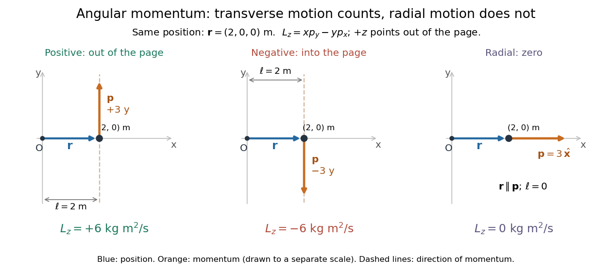
Positive, negative and zero angular momentum about the same origin
. Details. Fix an origin and nonrotating axes in an inertial frame. For a nonrelativistic point mass of constant mass , let be its position from and its mechanical momentum in that same reference frame. Its angular momentum is the cross productHere , , and is the angle between them. The right-hand rule gives the direction: curl from toward , and the thumb points along . Thus angular momentum is an axial vector, perpendicular to both position and momentum. Its International System of Units unit is . A point mass need not follow a circle to have angular momentum.[ref]
With rightward, upward, and out of the page, the cross product gives . TakeThen . Reversing the momentum makes ; radial momentum gives . The factor is the lever arm to the line through the particle parallel to its momentum.
For motion in the plane, plane polar coordinates give , with . ConsequentlyThe signed angular velocity is positive counterclockwise viewed from toward the plane, with measured in radians. Radial velocity does not enter the cross product. Under conservation of angular momentum, this relation predicts faster angular motion at smaller and constant areal velocity for consistently oriented swept area. That is the geometric content of Kepler's second law.
For several point masses, add their angular momenta about the same origin: . The origin matters: angular momentum under an origin shift explains why the same moving particle can have different values about two fixed points. The central axis of a momentum system and angular momentum decomposition about the centre of mass make this dependence useful.
In spatial dimensions, rotations have an antisymmetric tensor of conserved Noether charges when the dynamics is rotationally invariant. There are independent rotation generators. In three dimensions the tensor is equivalent to the axial angular momentum vector through .
Move the fixed origin from to , keeping the axes parallel and the inertial frame's velocity measurements unchanged. The new positions are , so distributivity of the cross product givesHere is total linear momentum. For the angular momentum example with , the new position is and . If total momentum is zero, angular momentum is independent of this origin shift. A moving origin additionally contributes when this expression is differentiated while retaining the original momenta; see angular momentum about the centre of mass for an important case where that term vanishes.
For nonzero total momentum , translating the origin by changes angular momentum to . The displayed line of origins makes this vector parallel to , equal to . The invariant cannot be removed by translation; if it is zero, angular momentum vanishes on this line.
A gyroscope is a rotating instrument whose rapidly spinning, nearly symmetric rotor provides a direction reference through its angular momentum. In an inertial frame, negligible external torque approximately preserves that direction by conservation of angular momentum. A transverse torque turns the angular momentum instead: the surprising sideways motion of a supported spinning wheel is precession. An ideal freely falling test gyroscope in general relativity has its spin undergo parallel transport along its timelike geodesic. Comparing that direction with distant reference axes measures Lense-Thirring precession; the direction need not remain fixed in arbitrary rotating coordinates.
A gyroscope direction reference is useful precisely because its direction can persist while its housing turns. A spinning-wheel precession experiment deliberately supplies gravitational torque to reveal how that persistence fails. The gyroscope vector geometry explains the direction, and slow steady gyroscope precession gives a numerical prediction with a check on its assumptions.
A flywheel's spin angular momentum must turn with the vehicle. The vehicle supplies torque to maintain this precession, and experiences the opposite reaction torque. With right-handed axes forward, left and up, a left turn has . A transverse flywheel with then produces body torque , opposing outward roll. Its magnitude is for turn radius . Reversing the flywheel reverses the effect.
A gyrocompass uses a spinning gyroscope and Earth's rotation to identify geographical north. In an ideal model whose axle is constrained to the local horizontal plane but free to turn about the vertical, the northward direction of the spin angular momentum is stable away from the poles; the opposite spin direction is unstable. A real settling instrument also requires damping. This is different from merely preserving an initial inertial orientation with a freely mounted gyroscope.
For a rapidly spinning gyrocompass with axle constrained horizontally, take azimuth positive from north towards west and positive spin angular momentum . In the terrestrial rotating reference frame, the vertical component of the torque equation, with zero external vertical torque, is . Here is the vertical moment of inertia and terms of order have been neglected. The small-angle approximation about gives simple harmonic motion with the displayed squared angular frequency. Linearizing about reverses its sign and gives an unstable equilibrium. At the poles this restoring effect vanishes. For a thin rotationally symmetric flywheel, the perpendicular axis theorem gives .
Choose a fixed support point and nonrotating axes in an inertial frame. All angular momenta, torques, and moments of inertia below refer to . Let point along the axle from toward the centre of mass, and let point vertically upward. Write for their angle. For a rapidly spinning symmetric top, the dominant angular momentum is , where is signed and is the axial principal moment of inertia. The sign of the axial angular velocity follows the right-hand rule.
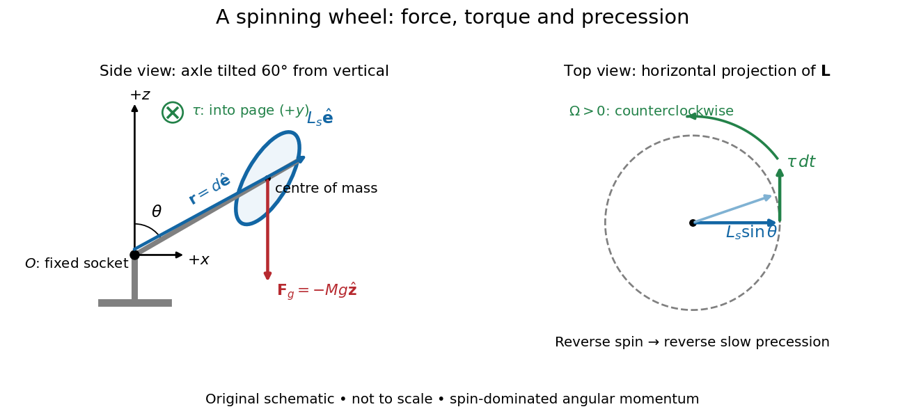
A fixed wheel support separates the downward gravitational force from the transverse torque and sideways precession
. Details. With mass , centre of mass distance , and constant gravitational acceleration , the gravitational force and its torque areAn ideal support applies a force at , so its lever arm and torque about vanish. At the instant the axle lies in the plane with a positive component, the gravitational torque points along . It adds toward , rather than along the downward force. The dot product identity shows why perpendicular torque changes direction without instantly changing magnitude. This vector balance and the slow-turning relation are developed in Chapter 20: Rotation in space (sections 20-2 and 20-3, equations 20.13–20.15).
For steady precession about the vertical, and . Equating the two cross products givesThe angular momentum tip traces a circle of radius : its sideways speed is . Both that radius and the gravitational lever arm contain , explaining its cancellation for . Exactly vertical alignment has zero gravitational torque and no distinguishable azimuthal precession to infer by this cancellation. Positive gives positive precession, counterclockwise viewed from above; reversing the spin reverses the slow precession. [ref]
11.4 Precession of a Gyroscope. University Physics Volume 1, section 11.4, equation 11.12 and the torque and precession-circle derivation
Purdue's Bicycle Wheel Gyroscope demonstration uses a bicycle wheel on a long axle, with a ball at one end seated in a freely rotating socket on a heavy stand. Spin the wheel by hand or with the supplied motor, seat the ball, and release the nearly horizontal axle. The readout is the axle sweeping around the vertical while the wheel continues spinning. Compare with the stopped wheel, which falls when one end is released; reverse the spin with the same support and the precession reverses. These are the page's documented apparatus, presentation, and reversal checks. [ref]
Bicycle Wheel Gyroscope by Purdue University, Department of Physics and Astronomy. 1Q-30, apparatus paragraph, Directions, and Suggestions for Presentation; page updated 30 November 2023
An alternative in Physics Demonstrations by Julien Clinton Sprott (section 1.3, Materials and Procedure) suspends one axle end by stainless steel wire and a fishing-line swivel. The swivel allows precession without winding up the suspension. Sprott describes the axle bobbing as nutation and precession becoming faster as spin decreases. A suspended support can move, whereas the calculation here assumes a fixed ; use the socket version for the closest realization. [ref]
Bicycle Wheel Gyroscope (section 1.3). section 1.3, Bicycle Wheel Gyroscope: Materials, Procedure, and Discussion
A proposed quantitative extension is to record an overhead view of an axle marker against a fixed angle scale, together with a side view for . Time successive overhead passages to estimate ; count passages of a rim mark to estimate . Record the spin sense too. Measure and the centre of mass offset of the whole moving assembly, and determine its axial moment of inertia independently. Wheel, axle, support, release angle, and observation interval should stay the same between spin trials. Measuring both and distinguishes azimuthal precession from nutation; an overhead movie alone can miss the latter. These camera readouts and parameter checks are proposed here, not reported measurements from the demonstration pages.
For slow precession, compare with , and test whether reversing reverses with nearly unchanged magnitude. A brief interval minimizes spin loss from friction; repeat at several starting spin rates rather than interpreting an entire slowing run as one steady state. A suspension restoring torque governed by its torsion constant, socket friction, support motion, a misplaced centre of mass, and a push at release can all supply extra torque or change the initial conditions. The swivel reduces the twist that activates the suspension's torsion constant; it does not demonstrate zero torque.
Steady precession keeps constant; nutation changes while the axle may also precess. Sudden release generally excites both. A small initial drop is consistent with conservation of energy and conserved vertical angular momentum: some gravitational potential energy supplies the motion around the vertical, and the axial contribution to vertical angular momentum adjusts. Bearing friction may damp the bobbing, but an ideal undamped heavy symmetric top need not settle into steady precession. Chapter 20: Rotation in space explicitly distinguishes uniform precession from release transients and nutation (section 20-3, paragraphs following equation 20.15).[ref]
Chapter 20: Rotation in space. section 20-3: sudden release, nutation, and the small drop needed for precessional angular momentum
Model the assembly as a heavy symmetric top with a fixed frictionless support, a uniform gravitational field, and centre of mass on its symmetry axis. Assume constant spin, negligible damping, and initial conditions prepared for uniform precession of a heavy symmetric top. Large spin means the transverse angular momentum from precession is small: . Also require . A large spin rate alone does not select steady motion after an arbitrary release.
For an original illustrative calculation, stipulateThe transverse principal moments of inertia are about the pivot, including the parallel axis theorem contribution. These inputs giveThe ratio is small; the more direct angular momentum ratio is small too. These are model calculations, not experimental results.
Check the approximation against the existing exact uniform precession of a heavy symmetric top condition. Its total angular momentum isAt constant , differentiating this expression and equating it to the gravitational torque givesFor the slow solution can be evaluated without subtracting two nearly equal numbers:It exceeds by about . The other solution is about and violates the assumed slow precession; the quadratic's two roots must not be conflated. Its discriminant must be nonnegative for these steady solutions to exist.
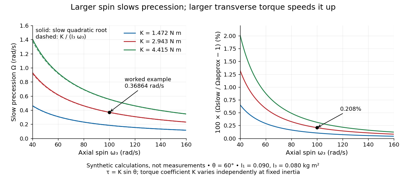
Synthetic steady-precession calculations: larger spin slows the drift and larger transverse torque speeds it up
. Details. The original curves hold fixed and vary spin and the imposed torque coefficient in . For gravity alone, ; the other curves are hypothetical changes in the transverse torque, not observations of this wheel. Solid curves use the slow quadratic root; dashed curves use . The second panel displays their relative difference. Increasing spin improves this approximation for the parameters shown. It does not remove nutation caused by inappropriate initial conditions.
Let a horizontal gyroscope have signed spin angular momentum along the axle. The disk's centre of mass is at and a counterweight is at . Gravity supplies torque . Since , steady horizontal precession gives the displayed signed vertical angular velocity. Neglect the axle's mass and the counterweight's axial spin moment of inertia. The zero-torque choice allows the axle to remain fixed. Moving the counterweight through this position reverses the gravitational torque and the associated slow precession.
For a rotor spinning about a principal axis with its support at the centre of mass, uniform gravity supplies no torque about that centre. With other external torques negligible, conservation of angular momentum preserves its direction in an inertial frame. A mount that permits free axis motion lets the housing rotate relative to that persistent direction, giving an orientation reference when external landmarks are unavailable. This is the useful limit opposite to the deliberately off-centre support in the spinning-wheel precession experiment. It supplies a direction, not a position or a full three-axis orientation from one axis alone.
For a small accumulated transverse torque about the centre of mass, the change in the direction unit vector is, to first order,Here is approximately constant over the short interval. Large angular momentum reduces drift for the same integrated transverse torque; parallel torque instead changes its magnitude. For , a constant transverse torque of over produces approximately , or , of direction change. This is another synthetic calculation. The persistent direction belongs to an inertial frame; its components can change in a rotating reference frame even with zero external torque.
A charged particle in a uniform field and an axially symmetric potential conserves the displayed canonical angular momentum, with the distance from the field axis and its charge. It follows directly by differentiating the expression and using the Lorentz force. For charge , the equivalent invariant is . A radial restoring force has no axial torque.
Consider particles of the same constant mass , interacting through equal-and-opposite central internal forces, with external forces for constant . About a fixed point , internal pair torques cancel and the external torque is . Hence and the displayed exponential decay follows. The same result holds for angular momentum about the centre of mass, because the moving-origin term vanishes. Unequal masses do not generally permit factoring out a single .
For a radial conservative force plus the magnetic-type force , the torque equals . Subtracting from ordinary angular momentum therefore produces a constant vector. Its dot product with is , so motion lies on a cone about that vector. At , ordinary planar central force motion is recovered. This is the classical radial magnetic monopole angular-momentum correction.
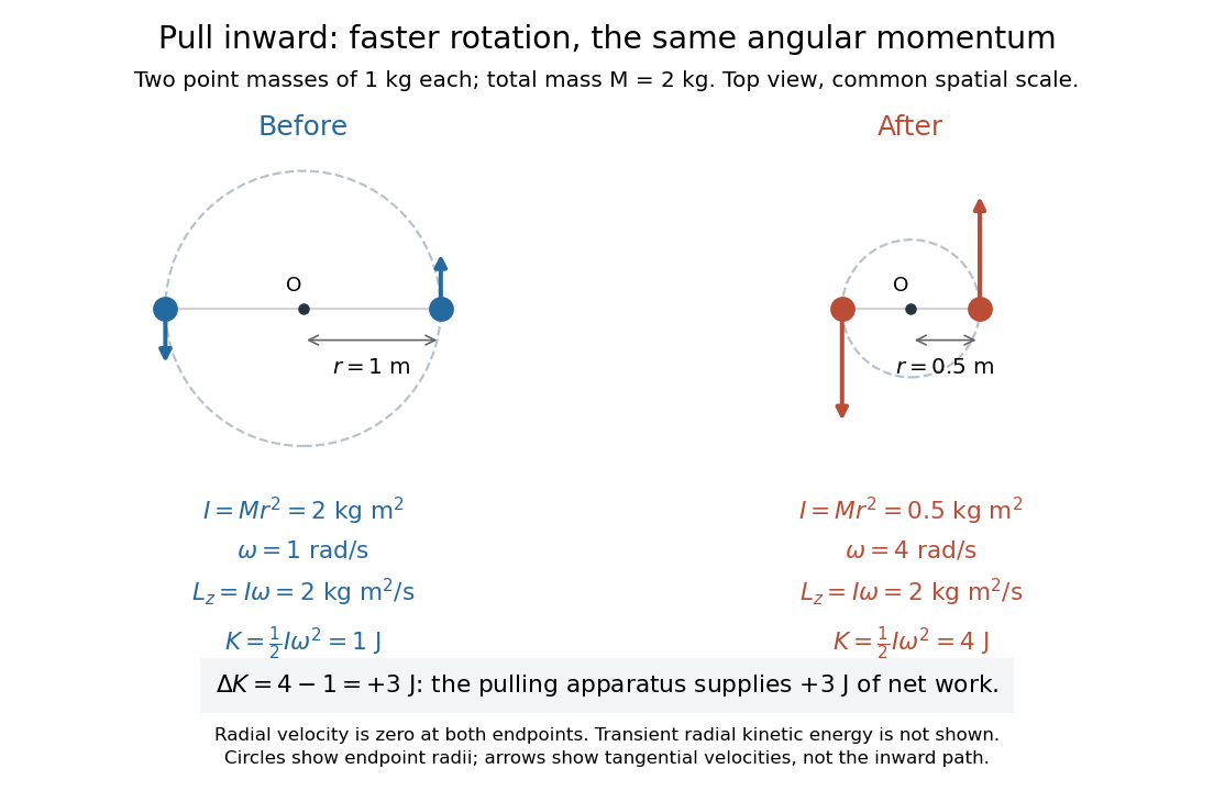
Conservation of angular momentum says that total angular momentum stays fixed when the net external torque about the chosen fixed inertial origin vanishes. Individual angular momenta and angular velocities can change. The radius change at constant angular momentum below makes this distinction visible: pulling two rotating point masses inward lowers the moment of inertia, raises the angular velocity, and supplies work that increases the kinetic energy.
Follow the same constant-mass point masses throughout, in an inertial frame, with all positions measured from a fixed origin . If the internal pair forces are opposite and central, meaning directed along each pair's separation, thenThus zero net external torque throughout an interval implies constant total angular momentum throughout that interval. A vanishing external torque component, such as , conserves the corresponding even when the other components change. This is the balance law for a fixed collection; angular-momentum flux must also be accounted for when matter crosses its boundary. [ref]
The central qualification is essential. Write for the internal force on member from member . Under Newton's third law, , but the sum of their torques isThis vanishes when is parallel to . Equal-and-opposite forces alone do not suffice: two opposite transverse forces with separated lines of action form a couple with nonzero torque. Cancellation of the internal pair torques, together with Newton's second law, proves the total balance above.
For one point mass under a central force about , gives . The force may still change the speed and kinetic energy; its zero torque preserves angular momentum. With nonzero , keeps the motion in a fixed plane. Choosing the axis perpendicular to that plane, governs its angular progress. This removes an unknown from the central-force radial turning point calculation and helps reduce the Kepler orbit to a radial problem.
There is a historical geometric version of this result. In Book I, Section II, Proposition I of the Principia, Newton proves that motion under a central force toward a fixed centre stays in a plane and sweeps equal areas in equal times, using successive central impulses and equal triangle areas. [ref]
https://en.wikisource.org/wiki/The_Mathematical_Principles_of_Natural_Philosophy_(1846)/BookI-II. Newton, Principia, Book I, Proposition I, Motte translation, 1846 edition
In the modern notation above, constant areal velocity is : the old geometric proof and the angular momentum calculation express the same invariant.For two equal point masses joined by a light tether of length , the central moment of inertia is . With conserved angular momentum , the rotational kinetic energy is . Slow, smooth contraction gives with the displayed leading tension. The exact radial correction is and , so the total work-energy theorem remains exact for non-quasi-static schedules too.
Place two equal point masses of each on opposite sides of a fixed origin, at equal radius , and let them share a signed angular velocity in a plane. Their total mass is and their moment of inertia about the perpendicular axis is . Radial pulling forces have zero torque about that origin, soTake an initial radius and angular velocity , and a final radius . ThenandThese are endpoint states with . During the pull, the full kinetic energy also contains radial motion: . Assume the pulling apparatus supplies all net work to the two point masses; the work-energy theorem then fixes its net work at , including any radial acceleration and braking. Each mass spirals inward during the pull, allowing its inward force to do positive work. Conservation of angular momentum therefore predicts the final angular velocity without requiring kinetic energy conservation. For an apparatus included in a larger system, its stored energy supplies the increase consistently with conservation of energy. OpenStax uses the same mechanism to explain a skater pulling her arms inward. [ref]
https://openstax.org/books/university-physics-volume-1/pages/11-3-conservation-of-angular-momentum. OpenStax, section 11.3: work during a change of moment of inertia
The rate at which angular momentum crosses a surface, including advection and stresses. With positive inward mass accretion rate, the net inward flux in a steady accretion disk is .
For unit mass in a central force with potential and conserved angular momentum , a radial turning point has zero radial speed and therefore satisfies
For unit mass, incoming speed , impact parameter , and potential energy , put . At closest approach, conservation of energy and conservation of angular momentum give the displayed radii and tangential speeds . Consequently and . These relations compare equal force magnitudes. The attractive radial case is a singular collision, so the speed-product statement does not extend to that endpoint.
Angular momentum transport moves angular momentum between locations through matter, stresses, waves, or fields. An accretion disk must transport angular momentum outward for most of its mass to move inward.
Torque measures a force's turning effect about a specified origin. The geometry in the angular momentum diagram applies with force replacing momentum: transverse forces give positive or negative torque, while a radial force gives zero. A longer perpendicular lever arm makes the same force more effective, explaining why pushing near the end of a handle is useful.
For a force applied at position from a fixed origin in an inertial frame, its torque, or moment of force, isHere , is the angle between position and force, and is the perpendicular lever arm. Direction follows the right-hand rule; in the plane , positive counterclockwise as viewed from . The International System of Units unit is . Although torque and energy have the same physical dimensions, torque is an axial vector and energy is a scalar; their roles differ.
For and , . Applying the same force at gives ; reversing it gives a negative torque; directing it along gives zero. More generally, sum to find the total torque about one common origin.
For a constant-mass point mass, the product rule and Newton's second law show why net torque changes angular momentum:The first cross product vanishes because its factors are parallel. For a collection with canceling internal torques, the remaining sum is external torque, giving conservation of angular momentum when it vanishes.[ref]
A nonzero torque can turn the direction of angular momentum as well as change its magnitude. Indeed, the dot product gives : a perpendicular torque changes direction without instantaneously changing the magnitude. This is the geometry behind gyroscope precession. For a rapidly spinning symmetric top with a fixed tip, centre of mass distance from the tip, mass , and spin-dominated angular momentum magnitude , the slow steady precession approximation gives , where is gravitational acceleration. [ref]
11.4 Precession of a Gyroscope. OpenStax University Physics Volume 1, section 11.4: Precession of a Gyroscope
This is an approximation with ; the uniform precession of a heavy symmetric top retains contributions omitted by the spin-dominated estimate.A rigid body's axial moment of inertia and a constant resisting torque give constant angular acceleration . Hence and the angular displacement is the displayed expression. Equivalently, the lost rotational kinetic energy equals the resisting work . The total number of revolutions is ; the number of whole revolutions completed is its floor function.
For positive angular velocity, a motor delivering constant mechanical power produces torque . With constant opposing kinetic friction torque , angular momentum balance gives the displayed equation and a steady speed . A small increase in speed reduces the driving torque below the friction torque, making this equilibrium stable within the model. The constant-power idealization is singular at exact rest and requires a separate starting regime in a real motor.
The time integral of torque about a specified origin equals the change in angular momentum about that origin under the usual fixed-origin inertial frame balance. Its units are , equivalently . For rotation about a fixed principal axis, the magnitude is .
The lever arm of a nonzero force about an origin is the shortest distance from that origin to the line through the application point parallel to the force. Its length is , with unit vector . Thus torque magnitude is , maximal at a right angle for fixed and , and zero if the line passes through the origin. Sliding the application point along that line leaves torque unchanged, since . The same perpendicular-distance construction gives angular momentum magnitude for a line parallel to nonzero momentum through the particle.
A pair of equal and opposite forces acting along distinct lines has zero resultant force but a nonzero torque. If acts at and at , the total torque about any origin is . Shifting that origin changes the moment by the cross product of the shift with the resultant force, which is zero. A prescribed couple therefore specifies a pure turning moment independently of its reference point. In Stokes flow it can drive a rotating sphere in Stokes flow without a directly imposed translational force.
Moment balance equates the rate of change of angular momentum to applied torques. A static slender rod obeys .
Areal velocity measures how fast a position vector from a chosen origin sweeps signed swept area. It connects a geometric picture of motion to angular momentum: a long position vector with slow transverse motion can sweep the same area per unit time as a short one with fast transverse motion. Constancy requires a dynamical condition, given by the torque criterion for constant areal velocity.
Choose a fixed origin in an inertial frame and a fixed plane through , with constant unit vector normal to it. For a differentiable trajectory in that plane, let be position relative to and its velocity. Positive swept area follows the right-hand rule about . In positively oriented Cartesian coordinates in the plane, and in plane polar coordinates with angle in radians,Here the dot product selects the normal component of the cross product. Motion away from or towards alone contributes no area. The signed specific angular momentum component obeysfor a constant mass . If is chosen along a nonzero conserved specific angular momentum vector, then and the familiar positive formula is . Reversing the orientation changes the sign; the instantaneous unsigned swept-area rate is .
Signed swept area counts the area traversed by a position vector, positively or negatively according to its direction of turning. For a continuously differentiable planar trajectory, its accumulated value relative to is the line integralA short segment contributes the oriented triangle area ; taking its time derivative gives areal velocity. Repeated turns count repeated area; a reversal subtracts it. Thus this quantity need not equal the area of the union of all previously swept regions. The origin matters: the relevant origin for Kepler's second law is the attracting focus of the ellipse, rather than its geometric centre.
Take an illustrative elliptic Kepler orbit with semi-major axis , orbital eccentricity and gravitational parameter , in consistent dimensionless units. Its semi-minor axis is , mean motion is , and specific angular momentum magnitude is . About the attracting focus,The two sectors below each span , giving . Near periapsis the short radius sweeps a wide angle; near apoapsis the long radius sweeps a narrow angle. Constant areal velocity therefore does not require constant angular velocity or constant speed.
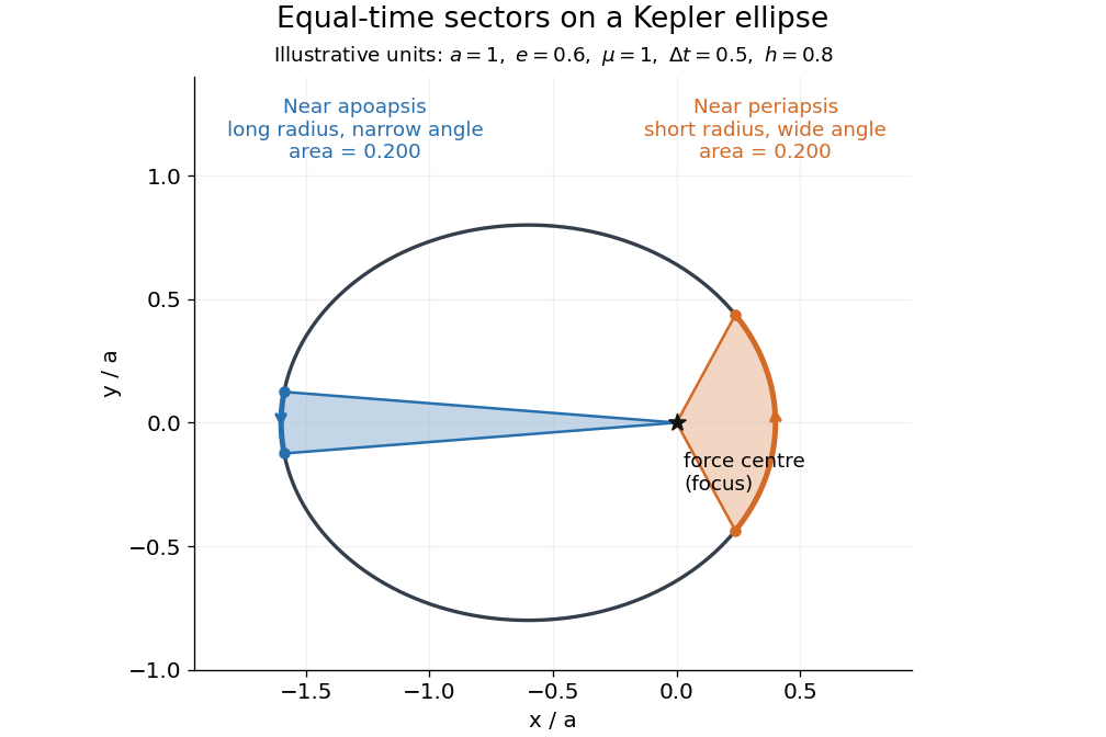
To compute the sectors without mistaking equal angles for equal times, parametrize the ellipse by eccentric anomaly :This follows by integrating . Kepler's equation gives , with mean anomaly measured from periapsis time . Consequently . The displayed sectors use mean anomaly intervals and , rather than equal eccentric anomaly increments.
Why infer an area law from astronomy? In the authored account The great Martian catastrophe and how Kepler fixed it by Owen Gingerich, a 13 August 1593 Mars observation has ecliptic longitude , against predicted and . These are Earth-based directions with a date, not measured Sun-based areas. The observer's armillary sphere used graduated circles and sighting arms to read declination; reversing it allowed a second reading. Comparing stars at different altitudes exposed refraction, and a planet-based check revealed an erroneous solar correction table. The apparent Mars distance signal had been contaminated by that correction. Johannes Kepler subsequently corrected the observer's Earth orbit, then tested Mars trajectories. The account describes typical angular errors of or less ( arcseconds): small residuals needed care.[ref]
The great Martian catastrophe and how Kepler fixed it by Owen Gingerich. pp. 51-53: Fig. 2, refraction checks, 13 August log table, Earth-orbit correction and angular errors
The Tufts class notes Kepler's Astronomia Nova and the Orbit of Mars explain the key limitation: an area requires a trajectory and distances, so Kepler's second law cannot be directly tested from angular observations alone. They describe checking the combined ellipse and area law against 28 dated observations around seven oppositions during 1583-1595, using an Earth model to predict Earth-based directions; agreement improved greatly but some discrepancies remained.[ref]
Kepler's Astronomia Nova and the Orbit of Mars. p. 20, items 3-5, and pp. 26-27, section IV.D: predictions, residuals and dependence of the area test on a trajectory
The inferential chain is useful today too: recover relative positions and times, compare swept areas, and ask what forces are compatible with their evolution. Agreement with equal areas supports zero torque about the chosen origin under the assumptions below; it alone does not identify an inverse-square law. Recovering the radial force also needs the trajectory and its timing, as in inferring an inverse-square force from Kepler laws. The two diagrams here are calculated examples, not the historical measurements.
An angular coordinate around the celestial sphere measured along the Earth's orbital reference plane. An Earth-based ecliptic longitude specifies a viewing direction; it does not by itself give a body's distance or its Sun-based position.
Assume a constant positive mass , a twice differentiable trajectory in the fixed plane, a fixed origin in an inertial frame, and Newton's second law for the net force. The product rule gives the short proofThe term vanishes. This is the planar angular momentum balance written in area language.[ref]
University Physics Volume 1. Section 11.2, equations 11.5-11.6: particle angular momentum and its torque balance
On a connected time interval, areal velocity is constant if and only if throughout. Since both position and acceleration lie in the fixed plane, the net torque has only that normal component. For , zero net torque is therefore equivalent to net force parallel to : its instantaneous direction is central, possibly inward, outward or zero. This diagnoses the net force along this motion, not its dependence on position or time elsewhere. Opposing transverse forces may cancel.
A central force about a fixed origin gives conservation of angular momentum, irrespective of its radial dependence: an inverse-square law is sufficient but unnecessary. With nonzero conserved angular momentum, fixes the orbital plane. Zero angular momentum gives radial motion and zero areal velocity; it does not select a unique orbital plane. The converse needs the fixed-plane assumption: a constant projected areal velocity in three dimensions only constrains one torque component. Also, makes the instantaneous torque vanish regardless of force and makes plane polar coordinates singular. A moving origin or changing plane requires additional terms.
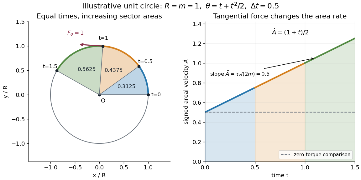
A path along a circle can have variable areal velocity. As an illustrative controlled trajectory, keep a point mass on a circle of radius with angleIts acceleration in polar coordinates and the required net force arewhere and are the radial and transverse unit vectors. A circular guide can supply the radial force, while a tangential drive supplies . HenceFor in illustrative units, the three equal time intervals , and sweep areas , and . Their difference comes from the transverse force's positive torque, even though the radius and path shape stay fixed. The area under each areal velocity graph segment equals the corresponding swept area.
A vector space whose coordinates are the components of a particle's momentum; a distribution in momentum space describes momenta rather than positions.
An integral over momentum space. For example, state counting in spatial dimensions uses a measure proportional to , whereas a relativistic Feynman integral commonly uses in natural units. The convention and any regulator must be specified. Independent loop momenta supply separate integration variables in a loop Feynman diagram; ultraviolet divergences and infrared divergences can require different regularizations.
Articles by others on the same topic



Momentum is a concept used in both physics and finance. ### In Physics: Momentum refers to the quantity of motion of a moving body and is calculated as the product of an object's mass and its velocity. The formula for linear momentum (\(p\)) is: \[ p = mv \] where: - \(p\) is momentum, - \(m\) is mass, and - \(v\) is velocity.