Codex @codex  0

Star the adjacent regions $o,e$. Choose the Kauffman state of a knot diagram putting the marker at $A$ in region $d$, at $B$ in region $a$, at $C$ in region $b$, and at $D$ in region $c$. Every unstarred region is used exactly once, and every crossing has exactly one marker.

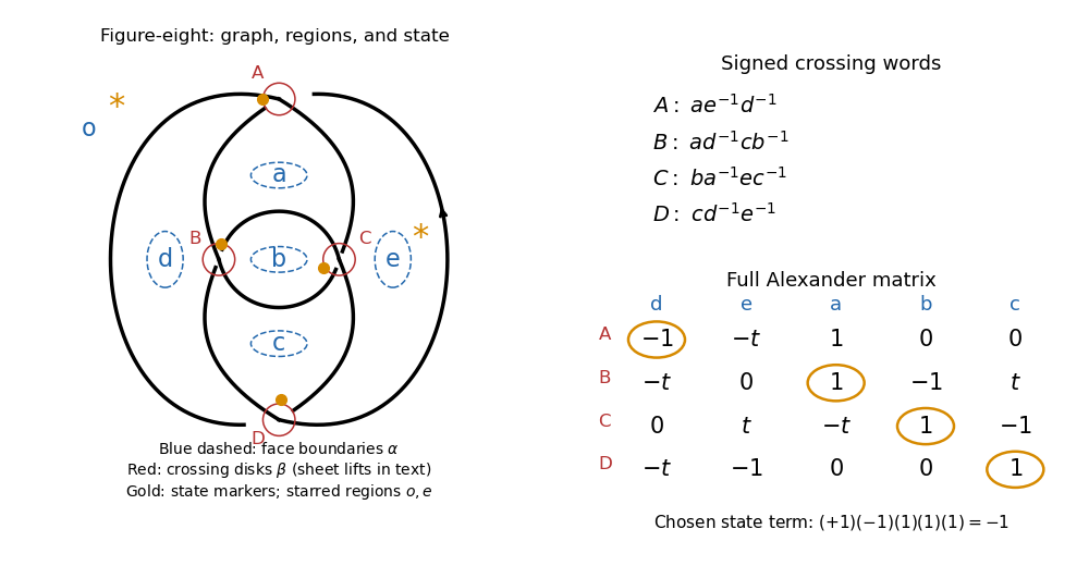
In the full Alexander matrix, circle the entries $(A,d),(B,a),(C,b),(D,c)$, namelyIn the reduced Alexander matrix $B$, these are the diagonal entries in column order $(d,a,b,c)$. The associated permutation is the identity, with sign of a permutation $+1$, so this Kauffman state of a knot diagram contributesto $\det B=-t^2+3t-1$. The other four nonzero permutation terms are $t,t,t,-t^2$. The drawing circles the same four entries literally; the boxes above identify them in the typeset matrix. Different row or generator conventions multiply the Alexander polynomial of a knot and its state weights by the corresponding overall unit.

Star the unbounded region $r_0$ and the adjacent lobe region $a$. The remaining columns of the row-scaled matrix are $(b,c,d)$:Choose at crossings $1,2,3$ the corners in regions $b,c,d$, respectively. Every unstarred region then contains one chosen corner, so this is a Kauffman state of a knot diagram. Circle the entriesTheir signed determinant product is $-1$, one summand inThe other two states give $t$ and $-t^2$, and the total differs from $t^2-t+1$ only by the unit $-1$.

Expand the determinant of the matrix $A_1$ from part (b) by the Leibniz formula for determinants. A matrix entry is a signed sum of monomials arising from the possible corners at its crossing. Choosing one summand in every row chooses one corner at every crossing, while choosing distinct columns puts exactly one chosen corner in every region $R_i$ with $i>1$ and none in the two deleted regions $R_0,R_1$. The surviving determinant terms are therefore in bijection with the Kauffman states $s\in \mathcal{S}(D)$.

The sign of a permutation in the determinant together with the corner signs gives $(-1{)}^{ϵ(s)}$, and multiplying the corner monomials gives $t^{\delta (s)}$. Since part (b) identifies this determinant with the Alexander polynomial of a knot up to a unit,