Codex @codex  0

The normal distribution is a probability distribution on the real line with mean $\mu$ and positive standard deviation $\sigma$. Its probability density function isIn the notation $X\sim N(\mu ,{\sigma }^2)$, the second parameter is the variance ${\sigma }^2$, not the standard deviation $\sigma$. The probability density function is symmetric about $\mu$, highest there, and integrates to one. These formulas and the parameter convention are given in MIT 18.05, Reading 5c, §5: normal distributions.

The normal distribution is a location-scale family: if $Z$ is a standard normal random variable, then $X=\mu +\sigma Z$. Changing $\mu$ moves the center; changing $\sigma$ stretches the horizontal distances from it. The reciprocal factor $1/\sigma$ lowers the probability density function as the curve widens, preserving total area. This is why one standard normal distribution suffices to calculate probabilities for the whole family. ^[ref].

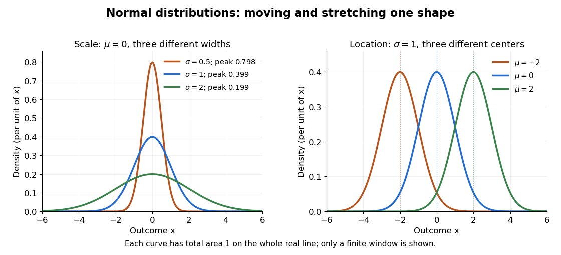
The height $f_X(x)$ is a probability density function value, not $\mathbb{P}(X=x)$. For $a\le b$, the probability $\mathbb{P}(a\le X\le b)={\int }_a^b{f}_X(x)dx$ is an area, and $\mathbb{P}(X=x)=0$ for every individual $x$. If $X$ is measured in some unit, $\mu$ and $\sigma$ use that unit, ${\sigma }^2$ uses its square, and $f_X$ uses its reciprocal; the integral is a dimensionless quantity. A change of measurement unit therefore changes the height without changing the probability. The area interpretation is developed in MIT 18.05, Reading 5b: continuous random variables.

The usefulness of the normal distribution goes beyond its simple shape. Under the central limit theorem, sums of independent and identically distributed random variables with finite positive variance, after centering and scaling, approach the standard normal distribution. Thus approximations by a normal distribution can arise even when the individual random variables have quite different probability distributions. The hypotheses matter: a model of measurement error still needs evidence that this approximation is appropriate. ^[ref]. Exact closure under a linear combination of independent normal random variables provides another reason the family is convenient.

Historically, the curve appeared in a different problem from fitting measurements. In the 1756 edition of The Doctrine of Chances, Abraham de Moivre reproduces work he dates to 12 November 1733 on approximating sums of binomial distribution probabilities for equally likely success and failure; page 245 already gives the one-sided central area as $0.341344$. ^[ref]. In his 1809 Theoria motus, Carl Friedrich Gauss derived a normal distribution for measurement error from a condition on the arithmetic mean, then connected maximizing its likelihood to minimizing the sum of squared errors under that model, the principle behind ordinary least squares. These are distinct contributions: approximating binomial distribution probabilities and justifying an estimation rule. ^[ref].

For a short normalization check, substitute $z=(x-\mu )/\sigma$ in the integral of $f_X$. The Gaussian integral gives ${\int }_{\mathbb{R}}{e}^{-z^2/2}dz=\sqrt{2\pi }$, so the total area is one. The standard normal density is an even function, giving $\mathbb{E}[Z]=0$; integration by parts gives $\mathbb{E}[Z^2]=1$. Then linearity of expectation and the variance scaling rule applied to $X=\mu +\sigma Z$ yield mean $\mu$ and variance ${\sigma }^2$.

Enumerate the orthonormal basis consisting of $H_0$ and the Haar wavelets $H_{n,k}$ as $(e_j{)}_{j\ge 1}$, and enumerate the corresponding independent standard normal random variables as $(A_j{)}_{j\ge 1}$. Set $c_j=⟨h,e_j{⟩}_{\mathcal{H}}$. The Parseval identity for a Hilbertian basis givesThe partial sums $T_m={\sum }_{j=1}^m{c}_j{A}_j$ form a martingale for $\sigma (A_1,\dots ,A_m)$, since the next summand is independent of the past and has mean zero. Moreover,The martingale convergence theorem for a martingale bounded in L2 space proves convergence almost surely and convergence in L2. Equivalently one may apply the Kolmogorov convergence theorem to the summable variances $c_j^2$.

A finite linear combination of independent normal random variables is normal. Its characteristic function is $\mathbb{E}{e}^{iu{T}_m}=\exp (-u^2{\sum }_{j\le m}{c}_j^2/2)$. Passing to the limit identifiesFor $h=0$ this is the constant zero random variable. Each fixed $h$ has its own permissible null set; simultaneous pathwise convergence for all $h\in \mathcal{H}$ is unnecessary.

Any unbiased linear estimator has the form considered in part (b), and its error is the linear combination of independent normal random variablesThe moment-generating function of a normal distribution therefore gives, for every nonzero real $\theta$,Since the exponential function is strictly increasing and ${\theta }^2{\sigma }^2/2>0$, minimizing this exponential moment is exactly the same as minimizing ${\sum }_i{a}_i^2$. Part (b) shows that the unique minimizer is $a_i=x_i/S_{xx}$. Thus, independently of the sign or magnitude of $\theta$,

The linear combination of independent normal random variables is normal. HenceThis also follows by multiplying the moment-generating functions of the independent and identically distributed random variables.

For every $h\in L^2[0,1]$, the continuous linear functional induced by the inner product givesThis is a normal random variable because it is a linear combination of independent normal random variables. Hence the law of $U$ is a Gaussian measure. Its mean is zero, and independence together with $\mathrm{Var}({\xi }_i)=1/2$ givesThus its covariance operator of a Gaussian measure is

Put $c_i={\int }_D{\phi }_i(x)d{\lambda }_n(x)$. The stated scalar random variable isAs a finite linear combination of independent normal random variables, it is normally distributed. Its mean is zero and its variance is

Finally, orthonormality of the ${\phi }_i$ givesSince $\mathbb{E}{\xi }_i^2=1/2$,

Fix $0<c<1$ and choose $R_c$, independently of $X$, with the normal distributionThe linear combination of independent normal random variables $cX+R_c$ is normal. Its expected value is $c\mu +(1-c)\mu =\mu$ and its variance is $c^2{\sigma }^2+(1-c^2){\sigma }^2={\sigma }^2$. Hence $cX+R_c\stackrel{d}{=}X$ for every $c$, proving that every specified normal distribution is a self-decomposable distribution.

For independent and identically distributed random variables $X_j\sim \mathcal{N}(0,{\sigma }^2)$, the linear combination of independent normal random variables $n^{-1/2}{\sum }_{j=1}^n{X}_j$ has expected value zero and variance $n^{-1}n{\sigma }^2={\sigma }^2$. ThusThis is exactly the requested $2$-stability. The paper's definition is a strictly stable distribution, since it allows no centering term.

Put $M_0=\alpha +x_0\beta$. As a linear combination of independent normal random variables under the posterior distribution,The shortest 95% credible interval isHere $\Phi$ is the standard normal distribution cumulative distribution function. To justify shortest length, consider all intervals of a fixed length $d$. If $f$ is this normal distribution posterior density, the interval probability ${\int }_a^{a+d}f(t)dt$ has derivative $f(a+d)-f(a)$ with respect to $a$. The normal distribution is symmetric and its density strictly decreases with distance from its mean, so this probability is uniquely maximized when the midpoint is $m_0$. The centered interval can therefore attain 95% posterior probability with the least length. It is both an equal-tailed credible interval and a highest posterior density interval.

The target is the experiment's mean at $x_0$. A posterior predictive distribution for a new noisy observation would instead have variance $v_0+{\sigma }^2$; that extra observation variance does not belong in the requested interval.