Past exam of the chemistry course of the year 1 of the natural sciences course of the University of Cambridge / 2025 / 5 / b / Solution

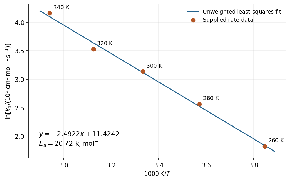
An unweighted least-squares Arrhenius plot using all five data points gives $\boxed{E_a=20.7\mathrm{kJ}\mathrm{mo}{\mathrm{l}}^{-1}}$. Define the dimensionless ordinate $y=\ln (k_1/k_{\mathrm{ref}})$ with $k_{\mathrm{ref}}=10^6\mathrm{c}{\mathrm{m}}^3\mathrm{mo}{\mathrm{l}}^{-1}{\mathrm{s}}^{-1}$, and set $x=1/T$. The model isFor increasing temperatures, the five ordinates are $1.82455$, $2.56495$, $3.13549$, $3.52636$, and $4.15888$. The linear regression slope and intercept areConsequently $E_a=-mR=20721\mathrm{J}\mathrm{mo}{\mathrm{l}}^{-1}$. The corresponding fitted $A=e^{11.4242}10^6=9.15\times 10^{10}\mathrm{c}{\mathrm{m}}^3\mathrm{mo}{\mathrm{l}}^{-1}{\mathrm{s}}^{-1}$. A two-point calculation using just the endpoints gives approximately $21.5\mathrm{kJ}\mathrm{mo}{\mathrm{l}}^{-1}$; the difference reflects the rounded, imperfectly collinear data rather than a unit conversion.