The first assertion is true. Each deletion removes a value with no support in an adjacent constraint domain. If a complete solution still used that value, the solution’s neighboring value would supply exactly such a support, a contradiction. By mathematical induction, AC-3 never deletes a value used by an original solution. An empty constraint domain therefore proves that no solution exists.
The second assertion is false. Take three Boolean variables with constraint domains and the binary constraints , , . Every value has the opposite value as support across each edge, so AC-3 deletes nothing and returns true. Yet and imply , contradicting . Arc consistency checks local support, not compatibility of all supports in one complete assignment.
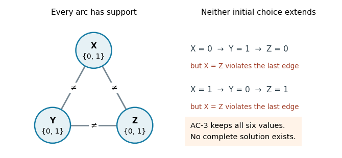
Every value has pairwise support, but following the three inequality constraints makes a complete assignment impossible
. Details. 
The third assertion is true under the usual explicit-input, constant-cost constraint-checking model. With variables, constrained pairs and maximum constraint domain size , AC-3 has time complexity in Big O notation. A revision costs ; each deletion can re-enqueue incoming arcs, and each constraint domain loses at most values, giving revisions including the initial arcs. For two-valued constraint domains, , so this is , linear in the explicit input size. This uses fixed-size relations, or already combined constant-time tests per pair. “Binary” normally describes constraint arity, not two-valued constraint domains; the latter restriction is the extra hypothesis needed here. As usual, initially empty constraint domains should be rejected before entering the algorithm, including isolated variables.
Interpret MyAC as doing at least one initial sweep, then repeating while the preceding sweep deleted a value. Its loop guard otherwise has no initialized truth condition. Both procedures apply the same support-based deletion rule, so both preserve every solution and terminate because finite constraint domains only shrink. Both return false on a detected empty constraint domain; neither successful return establishes satisfiability.
If a sweep changes no constraint domain, every directed arc has been revised against unchanged constraint domains, so all arcs satisfy arc consistency. Conversely, AC-3 places every potentially affected incoming arc back on its work list after a deletion. Its empty work list therefore also establishes arc consistency. When both run to successful completion, they compute the same arc-consistency closure, independently of revision order. To see maximality, any subdomains of the initial constraint domains that satisfy arc consistency survive every revision: each of their values retains a support inside those subdomains. Thus neither procedure can delete a value belonging to any such fixed point. Early failure may leave different intermediate constraint domains, but both failures correctly prove impossibility.
Their scheduling costs differ. AC-3 directs work toward arcs that may have lost supports, with standard time complexity . The full-sweep arc consistency method revisits all arcs after even one remote change. There are at most value deletions, so at most sweeps; a direct implementation including a scan for empty constraint domains costsIf empty-domain detection is maintained during revisions rather than rescanned, the familiar comparison is versus , apart from initialization. These are upper bounds, not exact costs on every input.
In practice MyAC is simple and may have low overhead or benefit from a fortunate sweep order. It can also waste many scans after changes propagate slowly opposite to that order. AC-3 incurs work-list bookkeeping but normally avoids those unrelated revisions. Both inherit the inability of arc consistency to decide arbitrary constraint satisfaction problems.
For a finite constraint satisfaction problem with variables, all complete assignments have depth when each step assigns one new variable. Thus the shallowest-solution property of breadth-first search offers no advantage: every complete solution is already at that depth.
Depth-first search with backtracking stores a path and pending choices, using auxiliary space with ordinary explicit choice bookkeeping, or when each level stores only a current value index. Breadth-first search may store an exponentially large frontier, up to partial assignments. Depth-first search can also combine naturally with immediate constraint propagation and undoing changes. The finite depth avoids the infinite-branch obstruction of unrestricted depth-first tree search. Neither traversal removes the possible exponential time complexity.
Write for the prescribed occupied cells, with . The source’s lowercase in its coordinate bound is read as the stated board size . If two prescribed queens already attack each other, no completion exists. Each model below correctly expresses that impossibility as well as consistent inputs.
Model 1: one Boolean variable per cell. Let indicate occupancy. Requireand impose for every two distinct cells sharing a row, a column or a diagonal. Equivalently, impose exactly one queen in each row and column and at most one on each diagonal. Explicit diagonal constraints areTogether with the total-count constraint and the attacking-pair binary constraints, these force exactly the intended boards. The count and diagonal-sum constraints are legitimate many-variable constraints; this model need not be binary.
Model 2: one variable per labeled queen. Let for . Enumerate and restrict for . For every , impose the binary constraintThere are exactly variables and distinct rows, so these are distinct queens. Labeling the prescribed queens does not lose a board completion: the queens are physically indistinguishable, and any completion can be labeled to give the prescribed ones those indices. It does create redundant assignments for the remaining labels.
Model 3: one variable per row. Let be the queen’s column in row . For every , requireand impose for every . These restrictions give queens, one per row; the all-different constraint on the columns gives one per column. For nonattacking queens on rows, exactly one per row is forced by the pigeonhole principle, so no solutions are lost. Inconsistent prescribed positions in a single row give incompatible unary restrictions. All three are exact constraint satisfaction problem encodings of the queens completion problem.
The conventional worst-case estimate is the backtracking leaf bound given by the product of the initial constraint domain sizes. Before exploiting any attacking-queen constraints, the three models give respectivelyModel 1 has binary choices. Model 2 has labeled queens with possible cells each. Model 3 has row variables with possible columns each. The rule of product gives the displayed bounds; assigning variables in one prescribed order avoids multiplying again by the number of variable orderings.
With mutually nonattacking prescribed queens incorporated as singleton constraint domains, the corresponding bounds improve toIn Model 1 only the prescribed occupied cells have been fixed in this estimate; immediate deletion of attacked cells tightens it further. In Model 3 consistent clues occupy distinct rows. If the clues are inconsistent, preprocessing can reject the instance immediately.
These are upper bounds on leaves, rather than exact attained counts for a fully specified pruning implementation. Ordinary backtracking rejects inconsistent partial assignments and often creates far fewer leaves; a stopped branch is itself a leaf even if not all variables were assigned. Such early leaves still obey the backtracking leaf bound, since distinct leaves describe disjoint nonempty families of full domain assignments when constraints are ignored. Counting only possible complete nonattacking assignments is a different question. For example, row/column restrictions alone reduce full assignments to at most in Model 3, but that number does not directly count failed partial leaves. Exact counts depend on variable ordering and constraint propagation, neither of which is specified.
Use Model 3 and keep every prescribed row at its prescribed column. Initialize one queen in every other row, and minimize the conflict countThis sum counts attacking pairs; is exactly a valid completion. A neighbor changes the column of one unfixed row. Evaluate such neighbors and move to one with lower , breaking equal choices arbitrarily. Minimizing , or maximizing , is hill climbing on complete domain assignments; these assignments need not yet satisfy the inter-row constraints. Fixed rows are never moved.
The min-conflicts algorithm chooses a conflicted unfixed queen and places it in a column giving the smallest conflict count against the other queens. Recomputing only the affected pair contributions makes a move cheaper than reevaluating every pair. Equal-cost moves can help cross plateaus; bounded sideways moves or repeated random starts of only the unfixed queens can escape some traps. These modifications still preserve the prescribed positions.
Return a board only after checking and every prescribed position. A local minimum with positive is not proof of impossibility. A queens completion problem may be unsatisfiable even when its prescribed queens do not attack each other; unrestricted restart policies give no finite worst-case success bound. If every row is fixed, simply validate the one board. For a guaranteed decision procedure use finite backtracking, possibly with constraint propagation, instead of relying on hill climbing.
Articles by others on the same topic
There are currently no matching articles.