Integrated master's degrees are included with their undergraduate entry courses. Oxford's preliminary examinations, moderations and Final Honour School parts are kept under their corresponding courses rather than treated as separate degrees.
The initial table of content was limited to the first level because it is larger than 1000 articles. There are 22929 articles in total. Expand a branch to load its children.
Official course page: www.ox.ac.uk/admissions/undergraduate/courses/course-listing/biochemistry-molecular-and-cellular
The listed headings are the five teaching threads.
Official course page: www.ox.ac.uk/admissions/undergraduate/courses/course-listing/biology
Students choose at least three of the four themes named in the directory; the themes are not separate degree programmes.
Official course page: www.ox.ac.uk/admissions/undergraduate/courses/course-listing/biomedical-sciences
Taught module choices; these determine the subsequent degree pathway.
Specialist options, short research project and specialist review. BA exit is in Neuroscience or Cell and Systems biology.
Optional fourth-year extended research project and review article leading to MBiomedSci in Neuroscience or Cell and Systems biology.
4 years. Award: MChem. Official course listing checked 2026-10-21. The directory says the course is under review; the listed structure is the currently published one.
Official course page: www.ox.ac.uk/admissions/undergraduate/courses/course-listing/chemistry
Core teaching and practical work.
Core and specialist teaching and practical work.
Research project.
Two shared programming/algorithms/proof-systems papers, discrete mathematics and probability, introduction to philosophy, and philosophical topics in logic and probability.
Algorithms and data structures, models of computation, group design practical, and options; philosophy teaching continues.
Advanced computer science and/or philosophy papers; project or thesis choices follow the joint course rules.
Solutions to all three questions of the University of Oxford examination held on 29 May 2023, including all 23 lettered parts. The paper allowed candidates to answer two questions; all three are solved here. Source release: released examination archive, member 2022/T/a16607w1.pdf, whose cover dates the examination to Trinity Term 2023. Question statements and the source illustration are omitted.
Let be the traversable squares and the exits. Sample the state space at the end of each complete round, so a live state is with . The given starting positions specify the initial state. The board and exits are fixed problem data, rather than changing components of the state space.
The rabbit has at most five actions: stay or move to one of its traversable orthogonally adjacent squares. A search transition model first applies that action, giving , and immediately checks for capture at . Otherwise hold fixed and apply the fox rule twice, checking for capture after each step. A capture is terminal failure; it must not be overlooked merely because the fox could subsequently move elsewhere. A surviving successor is . Equivalently, omit actions whose complete-round outcome is capture.
The goal test is the rabbit is on an exit after surviving the fox's entire turn: and no capture occurred in that round. Merely entering an exit before the fox moves is insufficient. Each surviving search transition model step has cost one when minimizing rounds.
Only legal moves are considered when applying the stated horizontal preference: try a legal horizontal step that reduces horizontal separation, otherwise a legal vertical step that reduces vertical separation, otherwise stay. If a blocked preferred direction is instead interpreted as forcing a stay immediately, the counterexamples below and all completeness and optimality conclusions remain valid.
Write . The ordered position pairs give at most states, or live states after excluding capture. Thus the usual Big O notation estimate is . An additional terminal-failure marker changes this by only one.
For distinguishable foxes, retain . Different foxes may share a square; none may share the rabbit's square in a live state. There are at most live position tuples, giving . These counts describe possible encodings; obstacles, starting positions and the fixed fox rule can make the reachable state space much smaller.
The branching factor of the search tree is at most five, so through depth it has at mostnodes in Big O notation. With no depth bound, the search tree can be infinite, despite the finite state space: tree search retains different action histories even when they end at the same position pair.
For a concrete repeating history, use a two-row, three-column board, indexed from zero, with the sole obstacle , rabbit at and fox at . Repeated rabbit stays leave the fox blocked horizontally with no vertical separation to reduce. Hence the same live state can repeat forever. An exit at is nevertheless safely reachable in one round.
Breadth-first tree search is complete and optimal for minimizing rounds. If a successful escape has finite length , there are only finitely many nodes at depths below , since the branching factor is at most five. Breadth-first tree search therefore reaches a shallowest successful node after finite work, even if other branches continue forever.
It is an optimal search algorithm because every search transition model step costs one round, so minimum depth is exactly the desired minimum number of rounds. The goal test must be applied to the surviving complete-round successor. Here a complete search algorithm guarantees finding an escape when one exists; it need not terminate on every unsolvable instance.
Depth-first tree search is neither complete nor optimal for minimizing rounds.
For incompleteness, use the two-row, three-column board from part (c), with exit . If stay is the first action explored, depth-first tree search follows the repeating state forever. Moving the rabbit down instead survives the round: under legal horizontal-then-vertical movement the fox moves to and then , leaving the rabbit safely at the exit. Thus a one-round escape exists but is never reached in this action order.
For nonoptimality, use an unobstructed one-row board with columns , initial fox column , initial rabbit column , and exits at columns and . Moving left once escapes at column with the fox at column . Moving right twice escapes at column with successive fox positions . A depth-first tree search that explores the latter route first returns two rounds although one suffices. This counterexample supplies an actual returned, suboptimal escape independently of the infinite-branch example.
Ignore the fox and obstacles when estimating the remaining number of rabbit moves. Define the heuristic functionThis is Manhattan distance to the nearest exit, a relaxation heuristic. Assume at least one exit; with none the instance is immediately unsolvable. The estimate is generally nonconstant and is not the perfect escape cost: obstacles can force detours, while pursuit can make an apparently nearby exit unreachable.
To prove it is a consistent heuristic, consider a surviving one-round transition from to . Let attain the minimum defining . The triangle inequality for Manhattan distance and the rabbit's move bound giveEvery successful terminal state has . This proves consistency with unit round costs; summing the inequality along any successful route also proves that it is an admissible heuristic. Failed transitions need no successor estimate because they are discarded.
Breadth-first tree search remains complete but is not optimal for maximizing the bonus. Completeness depends on the finite branching factor and a finite successful depth, not on the objective used to compare escapes.
Use the one-row, seven-square example from part (e). The one-round escape at column leaves the fox at column , so its graph distance to the exit, and hence the bonus, is . The two-round escape at column leaves the fox at column , giving bonus . The earliest successful node therefore has bonus when bonus is achievable. Breadth-first tree search orders by rounds rather than terminal graph distance.
Breadth-first tree search is complete and is still not bonus-optimal. Fix any deterministic rule for choosing among equally short fox routes; the completeness argument again uses only the finite branching factor. The unobstructed corridor of part (g) has unique shortest paths, so its fox moves are exactly the same under the new strategy. The one-round bonus is and the two-round bonus is , proving nonoptimality without any tie-breaking ambiguity.
If there is no route between fox and rabbit, the printed shortest-path rule needs a convention; letting the fox stay supplies a natural extension. The completeness argument is unchanged, and the counterexample above uses only connected squares. When the fox and rabbit initially belong to the same connected component of a graph, the shortest-path pursuit distance bound also makes every surviving branch finite. That additional property does not make the first escape maximize its bonus.
Depth-first tree search is complete under the stated initial reachability assumption, but is not bonus-optimal.
Let be the graph distance between fox and rabbit after round , with their initial graph distance. Initial reachability makes finite, and ordinary moves preserve membership in their common connected component of a graph. After the rabbit's next move, the triangle inequality gives intermediate separation at most . If that separation is at most two, the fox catches the rabbit that round. Otherwise the fox takes two steps along a shortest path, leavingThus a successful surviving history has at most rounds; if it does not escape by then, the next round captures it. The shortest-path pursuit distance bound excludes infinite live branches, even when the rabbit stays. Together with the finite branching factor, it makes the whole relevant search tree finite, so depth-first tree search eventually finds an escape whenever one exists.
For nonoptimality, take the corridor of part (g) and let depth-first tree search try left first. It immediately returns the one-round escape with bonus , whereas trying right twice earns . The decreasing separation proves termination, not optimality of the first returned escape.
In STRIPS, a state records the true ground facts; under the closed-world assumption, an absent fact is false. An action with positive preconditions , add effects and delete effects applies when , producing .
The given movement action adds the destination fact without deleting the old boat location. After its first crossing the boat can therefore be recorded at both banks, allowing physically impossible loading. Its source-bank symbol is also not a declared action parameter. Repair both issues by using the fully parameterized STRIPS actionHere excludes a vacuous same-bank crossing. The two static inequality facts already supplied suffice.
The given loading action has no capacity check. Consecutive loads can put arbitrarily many items aboard. Introduce a nullary planning fluent , true initially, and repair loading toUnloading must restore , as in part (c). Including the bank explicitly as an action parameter removes the other unbound action variable. Equivalently, instantiate separate east-bank and west-bank actions.
These repairs establish the planning state invariants that the boat is at exactly one bank, each item is either at one bank or aboard, and at most one item is aboard. The first two hold initially and are preserved by deleting the former location when adding the new one; the capacity marker permits loading only when no item is aboard. Grounding implicit location variables alone would not repair the missing delete effect or the missing capacity check.
The automated planning goal is the conjunction of the delivered-item facts:The boat need not separately be constrained to end west, although any successful plan with must bring the final item there before unloading it.
Use the STRIPS actionThe onboard precondition prevents inventing an item at a bank, and deleting preserves the item's unique location. Restoring preserves the one-item planning state invariant.
Each load starts with an empty boat beside an undelivered item. Each unload leaves that item west and restores the loading precondition. By mathematical induction on , after iteration the first items are west and the remaining items are east. Thus the automated planning goal holds after crossings and actions for . For , the empty plan already achieves the goal.
Replace the one-place marker by three nullary planning fluents , meaning that zero, one or two items are aboard. Initially only is true. Exactly one of these facts is maintained. No additional object constants are needed.
For compactness, define the common loading preconditionsand common unloading preconditionsThe four STRIPS actions areHere the first unloading removes one of two items, and the last unloading removes the sole remaining item; items do not require fixed seat identities. The movement action remains as repaired in part (a) and changes none of the occupancy facts.
The planning state invariant is true exactly when items are aboard. Every action changes the marker by the same amount as the actual onboard count, so it follows by mathematical induction from the initial empty boat. In particular, a third load is impossible.
Partition the items into successive groups of size two, with a singleton final group if is odd. For a pair on the east bank, executeFor a singleton , executeReturn the empty boat east between groups. Each group starts and ends with marker , and its items finish west, proving all preconditions and the final goal by mathematical induction over the groups. For there are outward journeys and crossings in total; is the ceiling function. Again needs no actions.
Keep the corrected one-place STRIPS model, replace the item constants and their initial typing facts by , and require all three west in the goal. The farmer travels with the boat, so the boat's bank also records where supervision is available. The new requirement concerns the bank being left: incompatible items may coexist at the farmer's current bank, but must not be left there together.
Here is a compilation using only ordinary positive STRIPS preconditions. Replace everywhere by , extending the item's possible locations toThe boat itself still has only bank locations, enforced by . Initialize a static relation for every and bank except . It states that two incompatible items at locations are not both on the bank about to be left.
Introduce planning safety certificates and , neither initially true. The following checking action grants a certificate:Add to the preconditions of . Every load, unload and move deletes both certificate facts. The other movement and capacity effects remain unchanged.
Deleting certificates on every location change prevents a stale safety check from authorizing a later unsafe departure. A certificate is granted only for the actual current locations and only when both incompatible pairs are separated on the departure bank. During a crossing the remaining bank is therefore safe; on arrival the farmer supervises the destination bank. This proves the required safety property by mathematical induction over crossings. The static facts are never changed.
Write for the three item constants, for the banks, for the corrected load, unload and move actions, and for instantiated with the items' actual current locations. A fully executable plan in the STRIPS model of part (g) isThus the seven crossings carry rabbit west, nothing east, fox west, rabbit east, carrot west, nothing east, rabbit west.
Immediately before those crossings, the items left on the departure bank are respectively . None contains an incompatible pair, so each displayed has its safety preconditions. Each loaded crossing carries exactly one item, and all three finish west.
For fair division, let and let the additive valuation of agent be . Use one variable per agent, with constraint domain , the power set of the items. Empty bundles are permitted in this original formulation.
Require pairwise disjoint sets:Each such binary constraint involves exactly . Require complete allocation by the single all-variable constraintFinally impose the envy-free allocation binary constraintseach on . The two directions for a pair use different agents' additive valuations and must both hold. These conditions give precisely an ordered set partition of the items that is an envy-free allocation.
Use one variable per item, with constraint domain . Its value is the recipient agent. Every assignment automatically allocates each item exactly once, so separate coverage and disjointness constraints are unnecessary.
For every ordered pair , imposeHere is an indicator function. The constraint involves every with ; one may formally give it scope , since zero coefficients make the other variables irrelevant. These constraints state envy-free allocation using the comparing agent's additive valuation on both sides. In contrast to part (a), they generally involve more than two variables.
With agent variables, each constraint domain has cardinality . Their total number of listed domain values is , while the Cartesian product of the domains hascomplete assignments before constraints.
With item variables, each constraint domain has cardinality . Their total number of listed domain values is , while their Cartesian product hascomplete assignments. These are raw domain-space sizes. The larger agent-variable space includes overlaps and missing items; imposing the allocation constraints reduces it to the same actual complete allocations represented directly by item variables.
Before using no-waste allocation to restrict the constraint domains, there is one constraint graph vertex for each of . Every distinct pair has a disjointness binary constraint, and also the two directional envy-free allocation constraints. Thus the constraint graph is the complete graph , with all ten edges.
The nonempty-bundle and no-waste allocation requirements are unary and add no edges. The original all-item coverage constraint has been removed because this variant permits unallocated items.
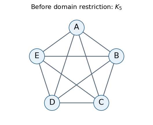
The allocation constraint graph before restricting the constraint domains
. Details. Restrict each agent to nonempty bundles of items that they value positively. Let the positive-value supports beThe residual constraint domains are , with sizes , respectively. The no-waste allocation and nonempty-bundle requirements are now built into these constraint domains.
If , every pair , is disjoint. Moreover, , so both envy-free allocation inequalities hold automatically because all values are nonnegative. Thus all three binary constraints disappear for the pairsThe only positive-support overlaps, and hence the remaining constraint graph edges, arewhere parentheses list the shared items.
Each listed pair really retains restrictions. For , , , , respectively, let both endpoints choose , , , : this violates disjointness while belonging to both residual constraint domains. The directional envy-free allocation inequalities are also individually nontrivial. For example, for , choosing and makes envious, while choosing and makes envious. The analogous shared-item comparisons apply on the other three edges.
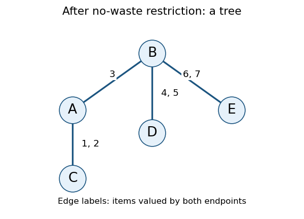
The residual allocation constraint graph; labels show shared positive-value items
. Details. The residual constraint graph is a tree, rooted conveniently at , with children and with a child of . Solve it by the tree-structured constraint satisfaction algorithm: enforce arc consistency from children toward their parents, then choose a surviving root value and select supported child values in the opposite direction.
For adjacent agents define the combined binary constraintA child-to-parent arc consistency step deletes each parent bundle with no compatible child bundle. Process the edges in the order , , , .
First, needs a nonempty subset of . Supporting reduces 's constraint domain toIndeed, leaves only for but gives value ; and leave no possible item for . Each of the four retained choices has a compatible choice for .
Next, supporting reduces 's constraint domain to all nonempty subsets of . To see why item cannot remain in 's bundle, a disjoint compatible bundle from would have to be , but then values its own bundle at and 's at least at . Conversely any nonempty subset of is compatible with .
Supporting next reduces 's constraint domain toIf held item , disjointness would force , whose value is below 's value for 's bundle. If holds but not , then , and needs value at least to avoid envying . If holds neither, supports every nonempty subset of .
Finally, supporting leavesThe removed choices contained both and , leaving no item for . Every displayed choice has a compatible choice for .
Choose , then supported child values, givingItems remain unallocated, which this variant expressly permits. To check every envy-free allocation inequality, the matrix of agents' additive valuations of these bundles, with rows and columns both ordered , isEach diagonal entry is at least every entry in its row. The bundles are nonempty, pairwise disjoint, and contain only positively valued items, so all remaining requirements hold.
Why does selecting supported children suffice? The residual constraint graph has no graph cycle, so different child subtrees have no constraints between them. Child-to-parent arc consistency has already ensured a compatible continuation below every retained parent value. Applying this observation recursively proves that the downward choices complete a solution without backtracking. With variables and maximum constraint domain size , the basic compatibility checks require time complexity in Big O notation, counting each binary constraint evaluation as one operation; evaluating bundle sums has its own input-dependent cost.
Articles were limited to the first 100 out of 22929 total.


