A probability density function must have integral one. For ,The restriction is essential: for the integral diverges and no positive normalizing constant exists.
For a moment of order with , integration of the probability density function givesThus the expected value and variance areThe cumulative distribution function on is . Its unique median satisfies , giving
For the independent and identically distributed observations, multiply the probability density functions. On the admissible parameter range , the likelihood function and log-likelihood areThese expressions presume that every observation lies strictly between zero and one; an observation outside that support would give zero likelihood under this model.
Write . The score function isSetting it to zero gives the maximum-likelihood estimatorThis lies above . The observed Fisher information isConsequently the log-likelihood is strictly concave throughout its domain. Its stationary point is the unique global maximum, not merely a candidate local maximum. Indeed the log-likelihood tends to minus infinity as either or .
The sample mean is . The method of moments equates this to the expected value from part (b):Hence the estimate is .
Here . The maximum-likelihood estimate and estimated standard error from the observed Fisher information areThe 95% Wald confidence interval is thereforeThe whole reported confidence interval lies in , though its lower endpoint is close to the boundary. With only four observations, the normal approximation underlying this Wald confidence interval need not provide accurate 95% coverage.
Keep the true parameter fixed and imagine repeatedly collecting four independent and identically distributed observations under the same model. Compute the maximum-likelihood estimate, its estimated standard error, and the Wald confidence interval afresh each time. The intended coverage statement is that approximately 95% of those random confidence intervals contain the fixed true parameter, provided the normal approximation is adequate.
After these particular observations have been collected, both endpoints are fixed. The frequentist statement does not assign 95% probability to the fixed parameter lying between these particular endpoints. Nor does the confidence interval describe the range containing 95% of future observations. The small sample makes the nominal 95% coverage an approximation whose accuracy is not guaranteed.
Both candidate models fit one parameter, but their parameter symbols have different meanings. For the exponential distribution in model B,Its second derivative is , so this is its maximum-likelihood estimate. The maximized log-likelihoods, including their normalization terms, areUse the corrected Akaike information criterion because is small relative to the number of fitted parameters:The correction is for each model, givingPrefer model A, whose corrected Akaike information criterion is smaller by . The ordinary Akaike information criterion also gives that ranking because the two models receive equal penalties. This compares the two proposed models; it does not establish that either is a correct description of the process. The usual corrected Akaike information criterion formula is a small-sample model-selection convention, rather than an exact finite-sample guarantee for these density families.
For the squared-denominator population map, a fixed point satisfiesThere is always the extinction fixed point . For a positive fixed point, divide by and use to obtainAt equality the candidate merges with zero and is not positive.
Differentiate the squared-denominator population map:At the positive fixed point, , so its fixed-point multiplier isSince , we have . A small perturbation obeys , and hence shrinks locally. Thus the positive fixed point is locally asymptotically stable by fixed point stability for an iteration.
This is a stage-structured population model with a census once per maturation interval. Only adults present at census contribute to the juvenile cohort at census ; each contributes new juveniles on average. Thus is an effective fecundity, including any survival of offspring needed to reach the next census. Juveniles present at do not contribute a separate birth term during this interval.
The term consists of juveniles that survive and mature into adults by the next census, so is their survival-to-maturity fraction. The term consists of surviving adults; is the adult mortality fraction per interval. All surviving juveniles leave the juvenile compartment in one step, adults remain adults, and there is no immigration or density dependence. The reproduction term is applied to adults counted at the start of the interval, rather than only to those surviving to its end.
Eliminate the juvenile variable from the stage-structured population model. Since ,The characteristic polynomial of this linear recurrence isso . The initial conditions give and , hence and . ThereforeThe alternating term records the initial imbalance between life stages; the growing term dominates eventually.
At a nonzero fixed point of the nonlinear stage-structured population model, the adult balance gives . Substitute into the juvenile equation and cancel :ThusBoth coordinates are positive precisely when .
The Jacobian matrix at the extinction fixed point iswith characteristic polynomialUnder , , whereas as . Hence its positive eigenvalueis greater than one. Its eigenvector can be taken with both components positive: choose . Thus there are biologically admissible positive perturbations that grow. The extinction fixed point is unstable by linear stability analysis for a discrete dynamical system.
Choose the diagonal matrix . Multiplying a vector by scales its th component by . ThereforeThe Euclidean norm objective for ordinary linear least squares on is exactly the weighted least squares objective, so the sets of minimizing vectors coincide. Zero weights simply discard the corresponding residuals.
Apply the least-squares normal equations to the transformed matrix and vector:or equivalentlyHere . A unique minimizing vector exists when the weighted design matrix has full column rank; the equations themselves remain valid without that assumption.
Using the paper's named weights , takeThe least-squares normal equations for weighted least squares becomeMultiplying by four gives and . Their determinant is , givingThus, to two significant digits, , with the slope measured in expression units per hour.
There is a wording convention to make explicit. Because the stated objective squares , the choice above gives the final two squared residuals one-quarter of the influence of the others. If “half as much” instead means half the coefficient of each squared residual, use . Then the least-squares normal equations aregiving and . Stating which quantity is halved resolves the ambiguity.
A BLOSUM substitution matrix is estimated from conserved, ungapped blocks of related protein sequences. Closely related sequences are clustered to reduce overrepresentation, and aligned amino acid pairs from different clusters are counted. Let be their normalized observed pair frequency, and the frequency expected from independent draws at the background amino acid frequencies. With unordered pairs, and for .
For BLOSUM62, scores are rounded half-bit logarithms of these odds:A positive entry means that the aligned pair occurs more often in related sequences than the independent-background model predicts; a negative entry means less often. Adding these scores accumulates evidence across aligned positions. A score is neither a percentage identity nor a direct substitution probability.[ref]
The statistics of sequence similarity scores by National Center for Biotechnology Information. The choice of substitution scores; The PAM and BLOSUM amino acid substitution matrices
A diagonal substitution matrix score measures enrichment over a background match, rather than simply rewarding an identical letter. tryptophan residues are comparatively rare, so a W–W match has a small chance background frequency . Its observed conservation produces a much larger ratio than the corresponding ratio for the more common leucine. The BLOSUM62 diagonal therefore awards W–W more than L–L. Both the background frequency and the observed pair frequency matter; rarity alone does not determine a diagonal score.[ref]
The number specifies the sequence-identity threshold used when clustering related sequences before deriving a BLOSUM substitution matrix. At 62%, sufficiently similar sequences are grouped and their within-cluster comparisons are excluded. Lowering the threshold merges more sequences, emphasizing comparisons across greater divergence.
Consequently BLOSUM80 is suited to closer relatives, BLOSUM45 to more divergent sequences, and BLOSUM62 is intermediate. The numbers do not specify a required identity of the query and target, nor a number of evolutionary time steps.[ref]
Amino acid substitution matrices from protein blocks by Steven Henikoff and Jorja G. Henikoff. pp. 10916–10917, clustering levels and performance across divergence
Read the ten residue–residue columns from the BLOSUM62 substitution matrix. In their order in the supplied sequence alignment, their contributions areThere are three gap positions, each incurring the stated linear gap penalty of four, including the leading gap. Therefore the alignment score is .
An affine gap penalty charges a larger opening cost than extension cost, reflecting that a single insertion or deletion event can span several residues. For a gap of length , explicitly chooseThe supplied sequence alignment has two gap runs, of lengths one and two. Its residue–residue score remains , so this choice givesMore generally, this affine gap penalty convention gives . There is no unique numerical rescore until opening and extension costs are chosen. A concave length-dependent gap penalty can make very long gaps progressively cheaper per added residue; distinct terminal gap penalties can accommodate incomplete sequence ends. Each choice encodes a different assumption about insertions, deletions or sequence completeness.
Use global sequence alignment, for example the Needleman-Wunsch algorithm with an appropriate substitution matrix and gap penalty. The two full-length globin proteins are related by orthology and are from closely related species, so the expected correspondence extends across both complete sequences. Unmatched ends should normally contribute to the score rather than being discarded.
With a linear gap penalty of magnitude , the dynamic programming entry is the best score for the first and residues. It satisfieswith , , and traceback from . An affine gap penalty uses separate match and gap states.
Use local sequence alignment, such as the Smith-Waterman algorithm, to compare the globin fragment with the matching region of each full-length target. A global sequence alignment would penalize long target flanks absent from the fragment. For a linear gap penalty the dynamic programming recurrence includes a restart option:Initialize boundary entries to zero, start traceback at the largest entry anywhere, and stop at zero. If the entire query is known to be valid and must be retained, fitting sequence alignment is a suitable refinement: align the whole fragment while leaving target flanks unpenalized.
First check the sequence alphabet: the prompt calls the targets “genes”. If the FASTA format file contains DNA rather than protein, translate the relevant coding sequences into amino acids before a protein-to-protein sequence alignment. If coding frames are unknown, search translated frames. A file in FASTA format specifies storage syntax, not whether the contents are nucleotides or residues.
The gain comes from avoiding a full dynamic programming table for every target. BLAST searches for short, sufficiently high-scoring word matches between query and database, then extends promising seeds. Modern versions reserve expensive gapped refinement for candidates passing earlier filters. FASTA sequence search similarly starts from short word matches, collects promising runs along alignment diagonals, and refines or joins selected regions. Word lookup and database indexing make candidate discovery inexpensive compared with considering every pair of positions.[ref]
Basic local alignment search tool by Stephen F. Altschul and others. pp. 403–406, word matches and hit extension
[ref]Improved tools for biological sequence comparison by William R. Pearson and David J. Lipman. pp. 2444–2446, FASTA search stages
These are heuristic algorithms: a good local sequence alignment can be missed if it has no acceptable seed, contains many interruptions, or is filtered before extension. Longer words and higher seed-score thresholds usually speed the search but reduce sensitivity; shorter words and looser thresholds recover weaker similarities at greater cost. Repetitive or compositionally biased regions can create many uninformative hits and erode both speed and specificity. No guarantee remains of finding the optimal sequence alignment for the chosen scoring scheme.
Thus the practical work depends on word length, thresholds, database composition and the number of hits. The speed-up is substantial on typical data, but does not establish a universal improved worst-case bound over : an input producing many candidate hits can still require extensive refinement.
A phylogenetic epoch is a time interval between successive branching events during which the number of ancestral branches is constant. Read backward from the four sampled leaves: there are four branches until the first merger, then three until the next, then two until their common root. Write the random durations as , with expected values .
The original solution diagram below places time horizontally and labels each branch by its number of descendant leaves. Type A is the pectinate topology; type B is the balanced topology. The coloured time strips identify the three phylogenetic epochs; their drawn widths are schematic, not estimated times.
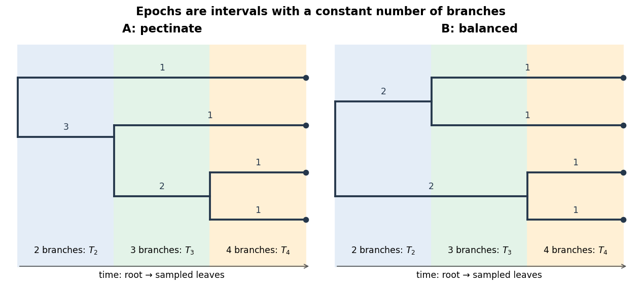
Epochs and descendant counts for four sampled lineages
. Time runs from the common root to the sampled leaves. The two panels distinguish the three-plus-one and two-plus-two root splits; numbers on branches count sampled descendants. Details.
Count the number of descendant leaves on each branch during each phylogenetic epoch. From the tips backward, both topologies have branch-size lists during , then during . During , type A has and type B has .
Let be the total length of branches carrying descendant leaves. Adding the relevant phylogenetic epoch durations givesFor example, type A has one external branch and one three-descendant branch throughout , while type B has two two-descendant branches. In either case the total expected branch length is , a useful accounting check. The stem above the common root is excluded because mutations there would be shared by all four samples.
In the Yule process, each of branches gives birth independently at rate per generation. The next birth therefore has total rate . Its waiting time has an exponential distribution, so the mean phylogenetic epoch duration isFor the ensuing calculation use , and . This is the inter-event waiting-time convention requested in the question, including an observation interval with four branches. Stopping the forward process immediately when the fourth branch is born would instead leave a zero terminal interval and describe a different sampling convention.
For a haploid population with possible parents, each pair of ancestral lineages merges backward at rate in the Kingman's coalescent approximation. With lineages there are pairs. Hence the mean phylogenetic epoch duration isThus , and . For an autosomal sample from diploid individuals, replace the number of gene copies by , giving . A mitochondrial sample naturally uses a haploid maternal effective population size; the common factor cancels in the ratios below.
Under the stated topology probabilities, and . Averaging the branch lengths from part (b), the expected length producing the folded class isThe factor in type A includes both the one-descendant and three-descendant root branches. The expected length producing the class isWith a common mutation rate per unit branch length, it cancels from the ratio of expected counts in this folded site frequency spectrum:For the Yule process,For Kingman's coalescent,These are ratios of ensemble expected mutation counts, not the expected value of the random ratio in one tree. The stipulated topology weights apply to both processes, and their waiting-time rates depend only on the current number of branches.
The observed folded site frequency spectrum has a larger to ratio than either expectation in part (d), and is closer to the Yule process expectation than to the constant-size Kingman's coalescent expectation. Both models can nevertheless produce deviations in one finite sample, especially because all mitochondrial sites largely share one genealogy; this observation alone is not a formal model-selection result.
For the Yule process, one possible violation is a recent reduction in the per-lineage branching rate rather than a constant . Lengthening the terminal four-branch interval adds one-descendant branch length and therefore preferentially increases the class.
For Kingman's coalescent, one possible violation is recent population expansion rather than a constant effective population size. Backward in time, coalescence is slow in the large recent population and faster in the smaller ancestral population. The resulting long external branches tend to increase the class relative to the class.
A network null model is an ensemble representing a specified baseline against which to assess an observed biological network. It should preserve the features that would otherwise confound the test: at least the number of vertices and edges, and often the degree sequence, direction, edge type, or relevant spatial constraints. It should randomize the feature whose biological organization is under investigation. An ensemble that preserves that very feature cannot test whether the feature is unusual.
For example, test whether a measured protein-protein interaction network contains more closed three-protein interaction groups than can be explained by the interaction counts of individual proteins. Define vertices as the measured proteins and an undirected edge as a reproducible detected interaction, using a fixed assay threshold and treatment of duplicates. Preselect the triangle count as the test statistic. Generate many simple random graphs by degree-preserving edge rewiring, rejecting self-loops and duplicate edges, with enough accepted swaps and separation to obtain a well-mixed reference sample. This retains the observed degree sequence while disrupting higher-order association.
Compute the same triangle count for every reference graph. Compare the observed count with this distribution; an empirical upper-tail p-value can be reported as for suitably sampled reference graphs. Report the size of the excess as well as its tail frequency, and check sensitivity to the assay threshold and any required connectivity constraint. A significant excess is evidence beyond the chosen degree baseline, while assay bias or spatial organization omitted from that baseline can still explain it.
A generative network model specifies a mechanism for producing networks, such as growth with preferential attachment, and asks what structures that mechanism creates. A network null model is defined by its role as a comparison baseline. These roles can overlap: the same random mechanism can be a proposed biological explanation in one analysis and a deliberately simplified null in another.
For the Erdős-Rényi model , choose the number of vertices and an edge probability . Visit every unordered pair of distinct vertices once and include its edge independently with probability . This construction gives a simple graph with expected edge count and mean vertex degree .
Increasing at fixed makes the graph denser, increases typical vertex degree and local clustering coefficient, and tends to shorten graph distances and improve connectivity. Increasing at fixed also increases the mean vertex degree; to retain a sparse comparison one instead decreases approximately as .
Its degree distribution is binomial distribution, approximately Poisson distribution in the sparse large- regime, so it is not a scale-free network. Connected realizations can have short average shortest path length, but their clustering coefficients are not elevated above the random baseline they themselves define. Thus they are not small-world networks under the high-clustering convention, although “small world” is sometimes used more loosely to mean only short distances.
For the Watts-Strogatz model, choose vertices on a ring, an even initial vertex degree , and a rewiring probability . Connect each vertex to its nearest neighbours on each side. Consider each original clockwise edge once: with probability , retain its starting endpoint and replace its other endpoint uniformly, excluding self-loops and duplicate edges. The edge count remains , although individual vertex degrees change.
Increasing at fixed lengthens unrewired-ring graph distances. Increasing adds edges and shortens distances. Increasing introduces shortcuts, sharply reducing average shortest path length at first, then progressively reducing the clustering coefficient by destroying local triangles.
The small-world network regime occurs at intermediate with sufficient shortcuts, substantial clustering, and . At distances are long; near the clustering advantage disappears. The degree distribution remains concentrated around , so this is not a scale-free network.[ref]
Collective dynamics of small-world networks by Duncan J. Watts and Steven H. Strogatz. pp. 440–441, construction and dependence on rewiring probability
For the Barabási-Albert model, choose a connected seed graph on vertices, the number of new edges per added vertex, and a final size . A complete seed with suffices. Add one vertex at a time, attaching it to distinct existing vertices selected with weights proportional to their current vertex degrees. Exclude duplicate edges and self-loops.
Increasing creates a larger network and permits older hubs to grow. Increasing makes the graph denser, with asymptotic average vertex degree , and tends to shorten graph distances. The seed affects early structure and the oldest hubs; standard linear preferential attachment gives a robust large-size tail exponent.
Its asymptotic degree distribution is , so it is a scale-free network. Hubs produce short average shortest path length, but elevated clustering coefficients are not automatic: with a tree seed gives a triangle-free tree, and clustering decreases with size in the standard model. The strict clustered small-world network property is therefore not guaranteed.[ref]
Emergence of scaling in random networks by Albert-László Barabási and Réka Albert. pp. 510–511, growth, attachment and degree exponent
The supplied adjacency matrix describes a four-vertex cycle graph, with every vertex degree equal to two. Degree-preserving edge rewiring is random, so it does not determine one unique labelled output adjacency matrix. For example, replace edges and by and , retaining and . This valid switch gives, in order ,Each row still sums to two. Under the simple graph convention, all allowed outputs have the same unlabelled four-cycle topology: there are three possible labelled four-cycles. A rejected switch or later return can also leave the original adjacency matrix.
It is not a scale-free network. Its degree distribution is concentrated entirely at degree two, with no power-law tail; degree-preserving edge rewiring cannot change that.
The diagram has all possible undirected edges except : it is a complete graph on five vertices with one edge removed. Therefore and each have three neighbours, while each have four.
The neighbours of and form a triangle, so their clustering coefficients equal one. Each of has five of the six possible neighbour–neighbour edges, giving . The nodal average shortest path length is . All graph distances equal one except , henceAveraging the nodal quantities givesThe ordered-pair distance sum is , and the graph diameter is two.
If the intended unnormalized “small-worldness” is the ratio of clustering to path length, the computed quantities giveThat ratio has no universal threshold for identifying a small-world network. The standard reference-normalized small-worldness, , cannot receive a numerical value when no reference is specified and the question forbids using a network null model.[ref]
The graph has high clustering and short paths in the descriptive sense. With nine of ten possible edges, however, those properties follow directly from its near completeness; they do not by themselves establish small-world network structure relative to a reference. This distinguishes the metrics that can be computed directly from the stronger classification that requires a stated convention.
Let be the displacement in step , so the random walk position is . The single-step expected value and second moment areBy linearity of expected value, . The steps are independent random variables, so for , . Expanding the square gives the mean squared displacementThese are ensemble expected values; the empirical average over a finite number of independent cells fluctuates about them. The expected mean squared displacement itself does not depend on .
For unbiased one-dimensional diffusion, the mean squared displacement is . With , compare this to the mutant expression:Therefore the mutant diffusion coefficient is
On a moving step, the largest speed resolved by the discrete model is the distance per interval,This is a step-averaged speed; the model does not specify motion within the interval. Use the cell length in the stated Reynolds number formula. In consistent centimetre–gram–second units,Thus viscous effects dominate inertia overwhelmingly. The surrounding flow is in the Stokes flow regime: sustained movement needs applied forces, and inertial coasting is negligible. Using radius rather than the specified length as the characteristic size would halve the Reynolds number, without changing that physical conclusion.
Take the membrane particle flux density to be positive from cytoplasm into the cell nucleus. With membrane permeability ,For fixed compartment volumes, conservation of mass and the absence of exterior flux giveSubtract the two concentration derivatives:This linear ordinary differential equation has solutionIts relaxation time is . Here has dimensions length/time, so has dimensions inverse time. A positive initial concentration difference decays monotonically toward zero; a negative one approaches zero from below.
The conserved total molecule amount fixes the final common concentration:Solve together with to obtainSubstituting the decaying concentration difference from part (d) supplies both explicit time dependences. The concentrations approach the volume-weighted initial average, which need not be the arithmetic average if the compartment volumes differ.
Yes, the data are centred. Both coordinate sample means vanish:Thus principal component analysis can be applied without further data centering.
Place observations in rows of the data matrix . Since the coordinate sample means are zero, the Gram matrix of its columns isThe sample covariance matrix is ; using divisor three instead changes eigenvalues by a common factor and leaves principal component loadings unchanged. For , the characteristic polynomial isFor the larger eigenvalue , the eigenvector equation gives , so . Normalize to unit Euclidean norm and choose . An orthogonal unit eigenvector for is . ThereforeThe sample variances of these principal components are and , respectively. Their principal component scores for observations areEither eigenvector may be multiplied by without changing its principal component direction or its variance. No coordinate standardization is applied here: that would instead be principal component analysis on a correlation matrix.
Articles were limited to the first 100 out of 208 total.
Articles by others on the same topic
There are currently no matching articles.