The initial table of content was limited to the first level because it is larger than 1000 articles. There are 4183 articles in total. Expand a branch to load its children.
Use Einstein summation convention, writing . The contraction of two Levi-Civita symbols givesThe last equality is the product rule. Recognizing the divergences and directional derivatives proves the curl of a cross product identity:
The divergence theorem states that, for a continuously differentiable vector field on a bounded region with piecewise smooth boundary and outward unit normal ,To apply it, first derive the divergence of a cross product using the Levi-Civita symbol and the product rule:In the second term the minus sign comes from interchanging the first two indices of the Levi-Civita symbol. The divergence theorem with now yields
Close the hyperboloid segment with the two disks at , and let be its interior. The flux through either disk is zero because . Thus the desired surface integral is the total outward flux through the closed boundary. Sincethe divergence theorem and cylindrical coordinates giveThe extra factor is the volume integral measure in cylindrical coordinates; omitting it would give the wrong flux.
For separation of variables, take and divide the reaction-diffusion equation by this product wherever it is nonzero:Each spatial term depends on a different variable and must be constant. Write and similarly for the other two factors. The Dirichlet boundary conditions give . A zero separation constant permits only a linear function and hence the zero solution; a positive value of likewise permits no nonzero function vanishing at both endpoints. The nontrivial choices are thereforeThe temporal ordinary differential equation isso, absorbing its constant multiplier into ,The superposition principle and completeness of the Fourier sine series give the stated threefold expansion with these factors. For an initial density , orthogonality also determines the constants:
The fastest temporal growth occurs for the lowest spatial eigenvalue, with . Its growth rate isFor a generic initial condition its coefficient is nonzero, so this term determines the long-time behavior. In fact, every nonzero, nonnegative initial density has , since the product of the three first sine eigenfunctions is strictly positive in the interior. ConsequentlyFor every term decays. At equality the first term is stationary and all higher terms decay: equality does not produce exponential growth. This is a reaction-diffusion equation threshold arising from competition between production and loss through the Dirichlet boundary condition.
The separation of variables solution with Dirichlet boundary conditions on the cuboid isThe constants are fixed by the initial density through Fourier sine series. The fastest term again has . When , its growth rate becomesThus the precise condition for no exponentially growing term isFor example, gives , while gives : either a sufficiently flat or a sufficiently elongated cuboid suppresses growth despite its unchanged volume. The function decreases to its minimum at , then increases without bound. Hence there are two positive threshold values, with growth only between them; equality leaves one stationary term and all other terms decaying.
The homogeneous linear differential equation can be written in divergence form:One integration gives . Therefore the two cases areIn each case the displayed functions have linear independence throughout the interval. Imposing both homogeneous Dirichlet boundary conditions forces : for , , and for , . This also establishes uniqueness for the inhomogeneous boundary value problem.
Choose the convention , where is the Dirac delta distribution, together with . The Green's function is continuous at and obeysThese conditions follow by integrating its differential equation across ; continuity prevents a derivative of the Dirac delta distribution. If and are homogeneous solutions satisfying the left and right boundary conditions, respectively, and is their Wronskian, thenFor take and . Their Wronskian is , and henceFor take and , giving andBoth formulas satisfy the endpoint conditions, continuity, and the unit jump directly. The unique solution of the boundary value problem isThe factor in the first formula matters: this Green's function is for the original monic differential operator, with ordinary measure , rather than for the operator multiplied by .
For , split the Green's function integral at . Writing and givesFor , the two integrals areSubstitution and simplification yieldAt both contributions vanish. At the bracket is . The differential operator kills and sends to , so this also verifies the inhomogeneous equation.
The exceptional integer is , because then the integrals contain . In this caseand the Green's function integral becomesHere , and . Explicitly and . Thus both exceptional and nonexceptional formulas satisfy the required boundary conditions.
Assume first that and are integrable functions, so that Fubini's theorem justifies changing the order of the two integrals. In the defining Fourier transform of the convolution, put :This proves the convolution theorem with the stated normalization:
Direct evaluation of the Fourier transform gives, for ,At the defining integral is the interval length, so . This also equals the continuous limit of the displayed formula.
The convolution is the length of the overlap of with . This overlap has length when and zero otherwise, so . The convolution theorem now givesThe value at zero is also the area of the triangular function, providing a normalization check on its Fourier transform.
The Translation property of the Fourier transform givesFor the remaining integral, the same Translation property of the Fourier transform identifies as the Fourier transform of . By the product form of the convolution theorem, with inverse normalization ,But is supported in , whereas the four translated triangular functions making up are all supported in . Their product is identically zero. Therefore the requested integral is for every real .
The matrix sending the standard basis vectors to the given columns isWith the Hermitian inner product, the squared column norms are , , and . The off-diagonal products areThus the columns form an orthonormal basis, so and is a unitary matrix. Here the operation maps the old basis vectors to the new vectors; the inverse coordinate change of basis uses .
The conjugate transpose reverses the order of matrix multiplication. Since and are Hermitian matrices,Consequently : the condition is exactly that the two matrices commute.
Take . Indeed the conjugate transpose isso the anticommutator is a Hermitian matrix. The original PDF, p. 6, supplies the factor that is corrupted in the local OCR.
Using the conjugate transpose and the Hermitian matrix assumptions,Thus is a Hermitian matrix, whether or not and commute.
Put , so . Because the Hermitian matrices commute,For every nonzero vector ,since is an invertible matrix. Thus and are invertible matrices, justifying the inverse in the definition of . The conjugate transpose of is . Since and commute, their inverses do too, andHence is a unitary matrix.
For the unitary matrix , . Therefore is a Hermitian matrix:Every positive integer power remains a Hermitian matrix, since . Its eigenvalues are real by the finite-dimensional spectral theorem. Equivalently, matrix similarity giveswhose eigenvalues are , where the are the real eigenvalues of .
Complete the square in the Hermitian matrix polynomial:For every nonzero vector ,Thus is a positive-definite matrix, so . In finite-dimensional spectral theorem terms, each eigenvalue isIf , the scalar polynomial has real roots of a polynomialAn allowed nonzero root can be an eigenvalue of , a Hermitian matrix which is also an invertible matrix, in which case has a zero eigenvalue. For example, , , gives . The weaker inequality does not force failure for every ; it removes the general positive lower bound. There is also the harmless corner , for which stays positive definite because is invertible, even though the strict discriminant hypothesis is absent.
For every vector , the Hermitian inner product givesThe norm vanishes only on the zero vector, so for every and . In contrast,is a nonzero nilpotent matrix. Multiplying a matrix by its conjugate transpose detects column norms; multiplying it by itself has no corresponding positivity property.
The cyclic property of the trace impliesTaking the matrix trace of the asserted equality therefore gives . For a positive integer over the complex numbers this requires . It is also sufficient: choose , or any two commuting matrices. Thus a finite-dimensional operator commutator cannot be a nonzero scalar multiple of the identity matrix.
The anticommutator condition and invertibility give the matrix similaritiesSince matrix trace is invariant under matrix similarity,Hence . Taking determinants in the first matrix similarity also givesSince is an invertible matrix, , and . In terms of eigenvalues, the same matrix similarity pairs each nonzero eigenvalue with , with the same algebraic multiplicity, so an odd number of them is impossible.
Termwise differentiation of the absolutely convergent matrix exponential series givesBecause and commute, also commutes with every power of and hence with . The product rule therefore givesDirect differentiation gives , and both initial values are . The uniqueness theorem for ordinary differential equations, applied to the finitely many matrix entries, implies . One can see uniqueness directly: the difference obeys and , soand the product is identically zero. At this yields
Let . The product rule and differentiation of the matrix exponential givewhere brackets are the operator commutator. Evaluating at zero gives , and . The Taylor series at zero is consequentlyIn particular , which also follows by multiplying the two matrix exponential series through quadratic order. For fixed finite matrices the remainder has the stated Big O notation in any matrix norm.
For a holomorphic function, the derivative supplied by complex differentiability must have the same value along real and imaginary increments. Those two computations giveEquating real and imaginary parts proves the Cauchy-Riemann equations:Conversely, if the first partial derivatives are continuous near a point and obey these equations there, real differentiability giveswhich proves complex differentiability under this regularity assumption.
The gradients of the real and imaginary parts have dot productand . At every point with , the two level sets are regular curves, their gradients are nonzero normal vectors, and their tangent directions are therefore perpendicular.
The printed phrase "at every point" needs this regular-point qualification. At a critical point with , the level sets may cross or fail to have a unique tangent. For example, gives and : at the origin the zero level sets are respectively the diagonals and the coordinate axes. Thus the valid conclusion is .
The Cauchy-Riemann equations determine the harmonic conjugate. Firstso integrates with respect to toNowand the second Cauchy-Riemann equation, , forces . HenceThe normalization at zero gives , so the required entire function is
For the first function, the complex exponential has no zeros, while the denominator has three distinct simple zeros. Thus there are . To examine infinity, substitute :The factor has an essential singularity at zero, and multiplication by a nonzero finite-order factor cannot remove it. Therefore of the first function.
For the second function, has simple zeros at . At zero, its Taylor series givesso . Every other is a double pole, since the numerator is nonzero there. There are no finite zeros, including after removal at zero.
At infinity the double poles accumulate. Equivalently, after , the function has double poles at tending to zero. Hence . The removable/pole/essential trichotomy for isolated singularities does not apply there; calling this an isolated essential singularity would be incorrect.
Put and . Partial fraction decomposition givesBoth terms admit a geometric series at . The local Laurent series is actually a Taylor series, since the center is regular:The nearest pole is , a distance from the center; the other pole is at distance . Thus the requested local radius of convergence is .
For completeness, specifying a Laurent series without a region can also mean either of the other maximal annuli. Expanding the first fraction in inverse powers and the second in positive powers givesExpanding both fractions in inverse powers instead givesThese are different Laurent series on different annuli, rather than extensions of the local Taylor series beyond its radius of convergence.
Away from , divide by the coefficient of to obtain the normal formThus are the only finite singular points. For a second-order linear differential equation, is a regular singular point if and extend analytically to . At these functions areand at they areEach pair is analytic at its respective point. Therefore .
Set . Then , and a Frobenius solution has the formIn the differential equation, the lowest power is , whose coefficient isThe indicial equation and its indicial roots are consequentlyTheir difference is not an integer, so the Frobenius method produces two independent series without a logarithmic term:Choose a branch of , or take for real solutions. A general local solution is by linear independence and the superposition principle. The analytic factors converge at least for , up to the next singular point at .
In the shifted variable , substitute the Frobenius solution into . Equating the coefficient of givesThus the linear recurrence relation, valid for , isFor the indicial root , this becomesFor the indicial root , rename the coefficients ; thenWith , the first terms of the two Frobenius solutions are
The generalized momentum of this Lagrangian isThe Euler-Lagrange equation therefore givesBecause has no explicit time dependence, the energy form of the Beltrami identity gives a conserved quantity . HereFor a direct check of conservation of energy, differentiate:This is the rest-plus-kinetic energy of a relativistic particle, in units with light speed one, plus its potential energy.
Write and , the initial Lorentz factor. The conserved energy from part (a) is . To emerge on the higher plateau with positive speed, the particle needs . HenceAbove this threshold, conservation of energy gives . The transmitted velocity is positive, soBelow threshold there is a turning point within the steep transition, where and . The particle returns to the lower plateau. Its final potential energy equals its initial value, so its final Lorentz factor equals but its direction is reversed:At exact threshold the limiting speed on the upper plateau is zero. This is the marginal case, not passage with positive outgoing speed. The ideal discontinuous potential does not specify the detailed trajectory at equality; a smooth transition can make the particle approach the top asymptotically. The final-speed formulas above cover the strictly transmitted and reflected regimes requested.
Take nonzero real trial functions with square-integrable and sufficient decay for integration by parts. For a compactly supported variation , the first variations areThe quotient rule for the functional then yieldsBy the fundamental lemma of the calculus of variations, stationarity for all such is equivalent toConversely, multiplying a decaying eigenfunction equation by and using integration by parts gives , so its Rayleigh quotient equals and its first variation vanishes. Thus the stationary values of the functional are the energy eigenvalues. The word "extrema" in the question includes stationary points here: higher eigenfunctions can be saddle points of the unrestricted Rayleigh quotient.
The Rayleigh-Ritz variational principle givesChoose an admissible trial family, calculate its Rayleigh quotient, and minimize over its parameters to obtain the best upper bound within that family. Equality holds for the exact ground state; a restricted family generally gives only an upper bound.
For the trial function, . The required Gaussian integrals areThe second formula follows by differentiating the first with respect to . Thereforeand division by gives the Gaussian variational bound for an attractive Gaussian well:This is a good trial family because it consists of smooth, positive, square-integrable functions decaying at both infinities. Each is an even function, matching the symmetry of the lowest bound state in this even potential, and the parameter varies its width. It also permits exact Gaussian integrals. Its Gaussian tail need not equal the exact exponential tail of a negative-energy bound state for the Rayleigh-Ritz variational principle to give a valid bound.
Differentiating the Gaussian variational bound for an attractive Gaussian well givesThus an interior stationary point obeysThe left side of the first equation increases strictly from zero to infinity, so there is exactly one such point. More explicitly,so is a strictly convex function on and is its global minimum. At that minimum the stationarity equation givesThere is a continuous limiting zero at , although at exactly is not a square-integrable function and hence is not an admissible trial. For a positive zero, division by and squaring gives , sois the unique positive zero. The other quadratic root is negative and inadmissible. Near zero,so the graph leaves the origin with slope , falls to its unique negative minimum, rises through , and grows as at infinity.
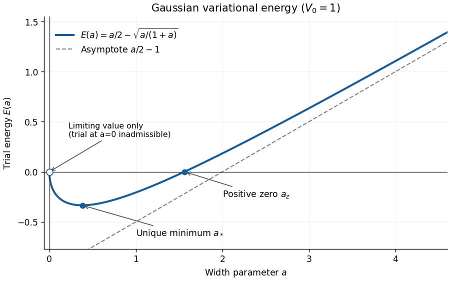
The Gaussian variational bound for an attractive Gaussian well at , showing its negative minimum and positive zero
. Details. 
By the Rayleigh-Ritz variational principle,Thus the attractive well supports a negative-energy bound state for every .
It is enough to choose an admissible parameter, without solving the minimizing equation. Take in the Gaussian variational bound for an attractive Gaussian well. The Rayleigh-Ritz variational principle giveswhere an explicit remainder isThe denominator tends to as , proving in Big O notation. More precisely the binomial series givesand thereforeThis is an upper bound on the exact ground state energy, rather than an assertion that the leading coefficient of its exact weak-potential expansion is .
Multiplication by gives the Sturm-Liouville formso the weight is . Use the weighted inner product and the Sturm-Liouville operator . Integration by parts gives its boundary form:The upper endpoint term vanishes by the Dirichlet boundary conditions, and the lower one vanishes for the regular solutions. More precisely, the radial Dirichlet spectrum in three dimensions identifies under the unitary transformation with on with zero endpoint values; this specifies the self-adjoint realization at the singular endpoint as well as proving the formal identity.
For eigenfunctions with different eigenvalues, the same identity gives . Taking real eigenfunctions proves the required orthogonality of Sturm-Liouville eigenfunctions.
Set . Direct differentiation gives , so . Finiteness of at zero requires , and the other endpoint gives . The Dirichlet eigenvalues are positive: integration by parts gives , and a nonzero cannot have zero right-hand side. Thus , and the second endpoint givesDefine by its limit. This is the radial Dirichlet spectrum in three dimensions with radius . Its weighted squared norm is .
Write the equation as with the positive Sturm-Liouville operator from part (a). A Sturm-Liouville eigenfunction expansion therefore gives , where weighted orthogonal projection givesHere the product-to-sum formulas reduce the integral to half the sum of the integrals of and . ConsequentlyAt , use the continuous limits of the terms. The coefficients are , so the resulting endpoint series converges. Completeness is the ordinary Fourier sine series completeness after . For an independent check, solving with zero endpoint values givesIts numerator vanishes at zero, and it has the same orthogonal projection coefficients. Positivity of proves uniqueness.
Articles were limited to the first 100 out of 4183 total.
Articles by others on the same topic
There are currently no matching articles.