Let , and . The chain rule gives and . Also , so . The killing term cancels, leavingThis is the explicit log-price scheme for local-volatility pricing equation. Under the risk-neutral measure, the corresponding log-price Itô formula givesThe logarithmic coordinate removes the stock-price factors from the diffusion coefficient, but retains the spatial variation of local volatility.
Write , and march backward from the terminal payoff. At the interior grid point useThe central finite difference spatial approximation and backward-in-calendar-time explicit Euler method giveHere , , and . At a far-left boundary use ; at a far-right boundary the call asymptotics are . These boundary values are inserted into the adjacent interior updates. Smooth-solution Taylor expansion gives consistency order in the evolution equation.
Refining space alone at fixed positive time step does not generally converge. The diffusion Courant number is , which grows by four at each halving of . For positive volatility it eventually violates the explicit diffusion stability restriction. The explicit log-price scheme for local-volatility pricing then amplifies grid-scale errors, rather than approaching the pricing solution.
The strike kink makes the failure concrete. At the terminal node , , while . Even a single step of fixed size gives , unbounded as if . Thus the problem is not cured by monitoring exactly at the money. A stable joint space-time refinement is required; the zero-diffusion case does not support the same diffusion argument and centered explicit advection has its own stability problem.
Refining time alone converges to the fixed-grid, spatially discretized solution, assuming the time-dependent coefficients and boundary forcing are suitably regular. In time-to-maturity , the grid values solve a finite system . For fixed , the explicit Euler method converges to this system as ; time-step error decreases to zero.
The spatial finite difference error remains. Thus the limit is not in general the exact continuous pricing solution: sufficiently small time steps reveal an error plateau of order under the usual smooth-solution assumptions. A truncated-domain boundary error also remains fixed unless negligible as stipulated.
Suppose the starting steps satisfy the nonnegative-weight restrictions given below, the volatility is bounded away from zero, and the coefficients and pricing solution have the regularity needed for the usual error expansion at the monitored positive remaining maturity. The combined refinement , preserves , improves the spatial drift restriction, and yieldsIf , put . Then , so the difference between successive refinement levels is . Consequently successive differences shrink by a factor of approximately four, giving second-order convergence in space and first-order convergence in time. If the leading coefficient happens to vanish, a faster rate or an irregular ratio is possible.
The volatility bounds alone do not guarantee that expansion: coefficient smoothness, stability and treatment of the nonsmooth terminal payoff matter. The statement applies at fixed positive remaining maturity after appropriate smoothing, not to Greeks at the terminal strike. If the starting diffusion Courant number is already outside the stable range, the proposed coupled refinement preserves that defect and does not establish convergence.
The option delta is a derivative in , not in . With , the logarithmic chain rule givesThus use for the delta hedge, and for option gamma. These formulas also identify the finite-difference option Greeks correctly on the equally spaced log-price grid.
There are two distinct accuracy statements. A smooth exact function has central first- and second-derivative truncation errors of order . But the computed values themselves have error under the coupled refinement. Without further control on its spatial variation,Therefore the value error bound alone guarantees only first-order delta accuracy and does not guarantee convergent gamma. For example grid error has a central first difference of order and a second difference of order one, despite second-order value accuracy.
If instead the scheme has a smooth error expansion with corresponding derivative bounds, both Greeks can retain second-order accuracy at smooth interior points. Hence reliable gamma is possible with additional regularity and a verified Greek refinement, but cannot be inferred merely from the value convergence in part (e). This qualification is important because the stated bounded-volatility assumption supplies no such error-derivative control.
Expand the update in part (b). Its trinomial tree weights areThey connect the current state to at the next time. Their sum is one, their mean increment is , and their raw second increment moment is . Thus they match the log-price diffusion to first order in the time step.
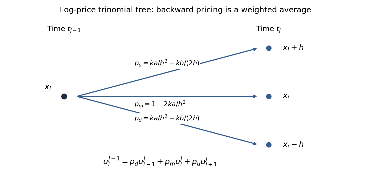
One-step log-price trinomial tree and its backward pricing average
. Details. 
All three weights are probabilities precisely when they are nonnegative:at every node and level. They are then automatically at most one. With positive , a simple sufficient uniform choice is and . If volatility vanishes at a node while drift does not, the centered weights cannot all be nonnegative.
Nonnegative weights make the backward update a convex combination, proving maximum-norm stability and monotonicity: interior errors cannot exceed the larger of the terminal and boundary errors. This is a sufficient stability condition, not an equivalence with every possible stability notion. For constant coefficients on an unrestricted or periodic grid, let and . The Fourier amplification factor isRequiring for every frequency gives and . Indeed, with , , so its two endpoint inequalities suffice. Probability weights require the stronger . The distinction prevents interpreting a merely Fourier-stable scheme with negative weights as a probability tree.
Articles by others on the same topic
There are currently no matching articles.