For a discrete-time martingale relative to the filtration , each is -measurable, , and for . The tower property then gives the corresponding identity conditional on any earlier time.
A bounded previsible process has measurable at time and . Its martingale transform is adapted and integrable, since each increment has absolute expectation at most . Moreover,Thus is a martingale, with .
For the Itô integral, begin with a bounded adapted step integrand on . Its integral is . Each summand has zero conditional mean. For , conditioning the cross product on makes its expectation zero. The conditional second moment of a Brownian increment is , henceApproximate the predictable integrand in by such step processes. The same identity makes their integrals Cauchy in and defines the limit; both its first and second moments converge. This gives the requested mean-zero result and the Itô isometry:
For the Ornstein-Uhlenbeck process, the deterministic integrating factor has no quadratic covariation with . The Itô formula therefore gives . Integrating and dividing by yieldsThe mean-zero integral and Itô isometry giveAt these formulas are read by continuity: , with mean and variance .
For the CIR model, let and use the usual positive parameters. Before a possible visit to zero, the derivatives of are and . Applying the Itô formula gives the Square root of a CIR diffusion:The PDF's claim under is false: that choice leaves the nonzero drift , which is not affine in . The actual interior cancellation condition is . Even then the principal square root is nonnegative and cannot be an unrestricted Gaussian OU process.
To give the intended corrected construction, let a signed process solve , with . The Itô formula givesWriting , with either sign chosen at zero, produces a Brownian motion; the diffusion term is . Thus is a CIR model with , while is reflected at zero. The reflection contributes local time of a semimartingale, so the interior SDE alone is not a global unrestricted OU equation. Its second moment is , agreeing with the CIR mean for that corrected parameter choice.
The requested mean under the parameters actually printed is still available without the false OU assertion. Taking expectation in the original CIR equation gives ; the stochastic integral has zero mean after the usual moment/localization justification. Consequently, for the printed choice as well as general admissible parameters,
Substitute the nonzero product into the Black-Scholes equation with continuous stock dividends and divide by on intervals where it is nonzero. The result isThe left side depends only on time and the right side only on spot, so both equal a constant . ThusThese are the separated solutions of the Black-Scholes equation. The zero solution is included separately, so division loses no relevant case.
For the unheaded parity request, the terminal difference of the power-call and power-put payoffs is . Under the risk-neutral measure, , where . The Gaussian exponential moment gives with . Discounting the difference proves power put-call parity:For this is the familiar dividend-adjusted put-call parity, .
If the value is independent of spot, both spatial derivatives vanish. The Black-Scholes equation reduces to , so , where is an arbitrary constant. A constant terminal payoff is therefore discounted at the interest rate ; its separation constant is .
For a time-independent value, . This is an Euler equation. Put to obtainFor , let . The roots areThey are distinct and real because , with one positive and one negative. The general stationary solution on is . There are no boundary restrictions in this subpart to eliminate either coefficient. In the degenerate case , the equation is first order: for its solutions are , while for only the zero stationary solution remains.
For the linear spatial factor, and . Hence and . Absorbing the constant into the time-factor amplitude gives . In particular a terminal claim equal to is worth , as expected for an asset paying a continuous dividend yield.
For , and . Thus , and all values with this fixed spatial factor areThis Power payoff in the Black-Scholes model calculation remains valid for any real on ; the specified nonzero exponent excludes the constant-payoff subpart. It also supplies the moment term in power put-call parity above.
Let , and . The chain rule gives and . Also , so . The killing term cancels, leavingThis is the explicit log-price scheme for local-volatility pricing equation. Under the risk-neutral measure, the corresponding log-price Itô formula givesThe logarithmic coordinate removes the stock-price factors from the diffusion coefficient, but retains the spatial variation of local volatility.
Write , and march backward from the terminal payoff. At the interior grid point useThe central finite difference spatial approximation and backward-in-calendar-time explicit Euler method giveHere , , and . At a far-left boundary use ; at a far-right boundary the call asymptotics are . These boundary values are inserted into the adjacent interior updates. Smooth-solution Taylor expansion gives consistency order in the evolution equation.
Refining space alone at fixed positive time step does not generally converge. The diffusion Courant number is , which grows by four at each halving of . For positive volatility it eventually violates the explicit diffusion stability restriction. The explicit log-price scheme for local-volatility pricing then amplifies grid-scale errors, rather than approaching the pricing solution.
The strike kink makes the failure concrete. At the terminal node , , while . Even a single step of fixed size gives , unbounded as if . Thus the problem is not cured by monitoring exactly at the money. A stable joint space-time refinement is required; the zero-diffusion case does not support the same diffusion argument and centered explicit advection has its own stability problem.
Refining time alone converges to the fixed-grid, spatially discretized solution, assuming the time-dependent coefficients and boundary forcing are suitably regular. In time-to-maturity , the grid values solve a finite system . For fixed , the explicit Euler method converges to this system as ; time-step error decreases to zero.
The spatial finite difference error remains. Thus the limit is not in general the exact continuous pricing solution: sufficiently small time steps reveal an error plateau of order under the usual smooth-solution assumptions. A truncated-domain boundary error also remains fixed unless negligible as stipulated.
Suppose the starting steps satisfy the nonnegative-weight restrictions given below, the volatility is bounded away from zero, and the coefficients and pricing solution have the regularity needed for the usual error expansion at the monitored positive remaining maturity. The combined refinement , preserves , improves the spatial drift restriction, and yieldsIf , put . Then , so the difference between successive refinement levels is . Consequently successive differences shrink by a factor of approximately four, giving second-order convergence in space and first-order convergence in time. If the leading coefficient happens to vanish, a faster rate or an irregular ratio is possible.
The volatility bounds alone do not guarantee that expansion: coefficient smoothness, stability and treatment of the nonsmooth terminal payoff matter. The statement applies at fixed positive remaining maturity after appropriate smoothing, not to Greeks at the terminal strike. If the starting diffusion Courant number is already outside the stable range, the proposed coupled refinement preserves that defect and does not establish convergence.
The option delta is a derivative in , not in . With , the logarithmic chain rule givesThus use for the delta hedge, and for option gamma. These formulas also identify the finite-difference option Greeks correctly on the equally spaced log-price grid.
There are two distinct accuracy statements. A smooth exact function has central first- and second-derivative truncation errors of order . But the computed values themselves have error under the coupled refinement. Without further control on its spatial variation,Therefore the value error bound alone guarantees only first-order delta accuracy and does not guarantee convergent gamma. For example grid error has a central first difference of order and a second difference of order one, despite second-order value accuracy.
If instead the scheme has a smooth error expansion with corresponding derivative bounds, both Greeks can retain second-order accuracy at smooth interior points. Hence reliable gamma is possible with additional regularity and a verified Greek refinement, but cannot be inferred merely from the value convergence in part (e). This qualification is important because the stated bounded-volatility assumption supplies no such error-derivative control.
Expand the update in part (b). Its trinomial tree weights areThey connect the current state to at the next time. Their sum is one, their mean increment is , and their raw second increment moment is . Thus they match the log-price diffusion to first order in the time step.
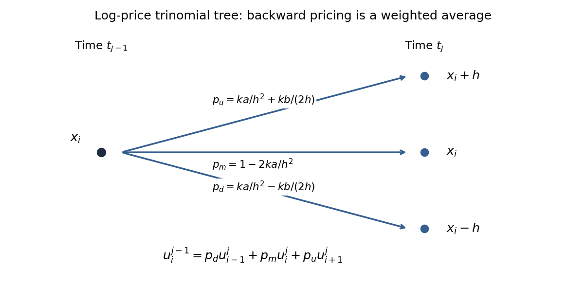
One-step log-price trinomial tree and its backward pricing average
. Details. 
All three weights are probabilities precisely when they are nonnegative:at every node and level. They are then automatically at most one. With positive , a simple sufficient uniform choice is and . If volatility vanishes at a node while drift does not, the centered weights cannot all be nonnegative.
Nonnegative weights make the backward update a convex combination, proving maximum-norm stability and monotonicity: interior errors cannot exceed the larger of the terminal and boundary errors. This is a sufficient stability condition, not an equivalence with every possible stability notion. For constant coefficients on an unrestricted or periodic grid, let and . The Fourier amplification factor isRequiring for every frequency gives and . Indeed, with , , so its two endpoint inequalities suffice. Probability weights require the stronger . The distinction prevents interpreting a merely Fourier-stable scheme with negative weights as a probability tree.
An instantaneous forward rate curve determines the unit-face-value zero-coupon bond through and . Integrating in maturity givesThe diagonal is the short rate, , and the continuous-time bank account has when . Therefore the discounted bond price martingale has valueUnder the risk-neutral measure of the Heath-Jarrow-Morton model, sufficiently integrable discounted bond prices are true martingales; without that integrability their stochastic dynamics initially establish a local martingale.
Since , multiplying the given bond dynamics by cancels the drift and gives . For an integrable discounted terminal payoff, the risk-neutral value process is the discounted-payoff martingaleFor an attainable claim this also follows directly from its self-financing discounted wealth being a true martingale, with terminal value . In a Brownian market, the Brownian martingale representation theorem provides ; a traded bond with nonzero diffusion exposure can hedge it by holding bond units, with the remainder in the bank account. Thus, under the usual attainability and integrability assumptions, this construction gives the replicated price as well as the risk-neutral pricing formula.
Because is -measurable,In a general Heath-Jarrow-Morton model, writing this value as requires an additional state-reduction assumption. The conditional expectation is valid without asserting that the short rate alone is the full state.
Assume the forward field is sufficiently differentiable in maturity to differentiate its deterministic and stochastic integrals. Moving along the diagonal adds the maturity derivative to the fixed-maturity dynamics:The Heath-Jarrow-Morton model no-arbitrage drift is , so . Equivalently, from the integrated forward equation,That drift can depend on the entire previous forward curve or driving path, rather than on the current scalar rate.
The short rate need not be Markov. For a concrete One Brownian factor does not imply a Markov short rate example, take the deterministic volatility . Its admissible risk-neutral drift is , andSubtracting the deterministic part leaves . The past of reveals its derivative , and . Yet is not determined by : the Gaussian covariance calculation givesConsequently the conditional law of the future depends on more than , proving failure of the Markov property for the scalar short rate. The enlarged pair is Markov. Special maturity-volatility structures, such as those producing a Vasicek-type short-rate diffusion, can instead admit a scalar Markov realization.
A credit rating is an agency's ordered assessment of an issuer's or particular obligation's capacity and willingness to meet its promised payments. Corporate and sovereign issuers are classified on letter scales, with finer notches, broad investment-grade and speculative-grade groupings, and default categories. Agencies such as Standard & Poor's, Moody's and Fitch also revise ratings as information changes; sovereign assessments involve public finances and institutional or political factors as well as debt-servicing capacity.
A credit rating summarizes relative creditworthiness rather than specifying an exact, immutable credit default probability. Historical defaults and migrations within rating classes can inform a statistical model. Assuming a homogeneous Poisson process within one class is a simplifying choice: it posits a constant event intensity and independent increments, neither of which follows merely from a shared rating. The credit risk model must also distinguish default frequency from loss given default severity.
The event that the first arrival exceeds is exactly the event . Thus for , and differentiation gives the exponential distribution density for .
For observed complete independent exponential gaps, let . The likelihood function is , and the log-likelihood has derivative and second derivative . Hence the unique maximum-likelihood estimator isAlternatively, observe unit-year increments . These are independent Poisson counts of mean . Their joint likelihood is proportional to , givingIt is unbiased, with variance . A zero observed count gives the boundary estimate zero, or the supremum as if the parameter space is restricted to positive rates.
The Poisson observation scheme and rate likelihood distinction matters when comparing the techniques. For a fixed observation horizon, conditional on the total number of events the event locations have a distribution independent of . Thus exact timestamps add no rate information to the total count under the homogeneous Poisson model; unit-interval counts already contain that total. The correct fixed-horizon likelihood includes the final unfinished waiting interval, and gives count divided by the full exposure, not by the sum of only completed gaps.
The first calculation instead stops after a fixed number of events, so its exposure is random. Its estimate has mean for and an infinite mean for , unlike the unbiased fixed-horizon count estimate. For its variance is , asymptotic to . There is no universally more informative sampling technique without specifying the stopping rule and exposure. Counts are sufficient and convenient for estimating a truly constant rate; timestamps additionally help diagnose departures from constant intensity or independent gaps.
The central limit theorem states that for independent identically distributed variables with finite mean and positive finite variance ,Applying it to the exponential gaps givesInvert the approximate central probability . For an observed positive total , an approximate 95% confidence interval isEquivalently its endpoints are , with a nonpositive lower endpoint replaced by the parameter boundary. This is a large- approximation; the exact gamma law of permits an exact interval if needed. It is a two-sided parameter interval, not a 95th-percentile annual loss estimate.
Let annual total loss be , with an empty sum equal to zero. The assumptions give a compound Poisson distribution. Conditioning on the count,The tower property and total-variance formula therefore giveThe term is the extra uncertainty in the number of defaults. Replacing it by zero would incorrectly treat that count as deterministic.
For sufficiently many annual events and an adequate normal approximation, the value at risk at confidence level is the compound-Poisson annual loss quantileThe supplied quantiles give , and . In particular a one-sided 95% annual loss quantile uses , not the from the two-sided 95% rate interval. If the expected loss is covered separately, the approximate unexpected-loss reserve is the second term, rather than the full quantile.
Estimate the rate from a suitable historical count/exposure or gap sample, then insert into the loss formula. The interval in part (d) measures rate-estimation uncertainty; for nonnegative loss mean it can be propagated to lower and upper approximate quantiles because the displayed expression is increasing in . Severity parameters also require estimation, so the rate interval alone is not a confidence interval accounting for every source of uncertainty.
Mean and variance do not determine the exact loss quantile. The actual distribution isFor nonnegative losses it has a zero atom at least , so if that mass exceeds its exact value at risk is zero. With a small rate or a strongly skewed severity distribution, a normal approximation can therefore be poor. A loan book with dependent defaults, rating migration or varying exposures also needs more than the constant-intensity independent-severity model. These are model qualifications, not deductions from the credit rating alone.
Articles by others on the same topic
There are currently no matching articles.