Past exam of the mathematics course of the University of Cambridge / 2006 / ii / Paper 1 / 13I / Solution

The fitted grouped-binomial logistic regression generalized linear model treats seasonal hits $H_i$ as independent $\mathrm{Bin}(n_i,p_i)$ variables, with $n_i={\mathrm{AB}}_i$ andThus the response supplied to glm is a proportion, and weights=AB supplies its binomial denominator; it is not a regression with equally precise seasonal averages. I(Age^2) forms the numerical square rather than using a formula operator. The estimates maximize $\ell (\beta )={\sum }_i[H_i{\eta }_i-n_i\log (1+e^{{\eta }_i})]$ up to a constant, where ${\eta }_i=x_i^T\beta$, $x_i=(1,a_i,a_i^2{)}^T$.

The observed negative Hessian is $X^{T}WX$, $W_{ii}=n_i{\hat{p}}_i(1-{\hat{p}}_i)$. Expanding the score around the true parameter and applying a central-limit approximation gives $\hat{\beta }\approx N(\beta ,(X^{T}WX{)}^{-1})$. The reported standard errors are square roots of the diagonal entries of this inverse; the binomial dispersion is fixed at one. Each z value divides the coefficient estimate by its standard error, and the reported two-sided Wald test uses a standard normal approximation under the corresponding zero-coefficient hypothesis.

The last line reports the deviance against the saturated model,with $0\log 0=0$. There are 22 seasonal observations and three fitted parameters, so 19 degrees of freedom. Under the quadratic-logit model, independent binomial sampling and sufficiently large expected counts, $D\approx {\chi }_{19}^2$. The value 23.345 gives an upper-tail probability about 0.22, no evidence of lack of fit at conventional levels. This approximation and the independence assumption should not be confused with an exact test of a player's ability.

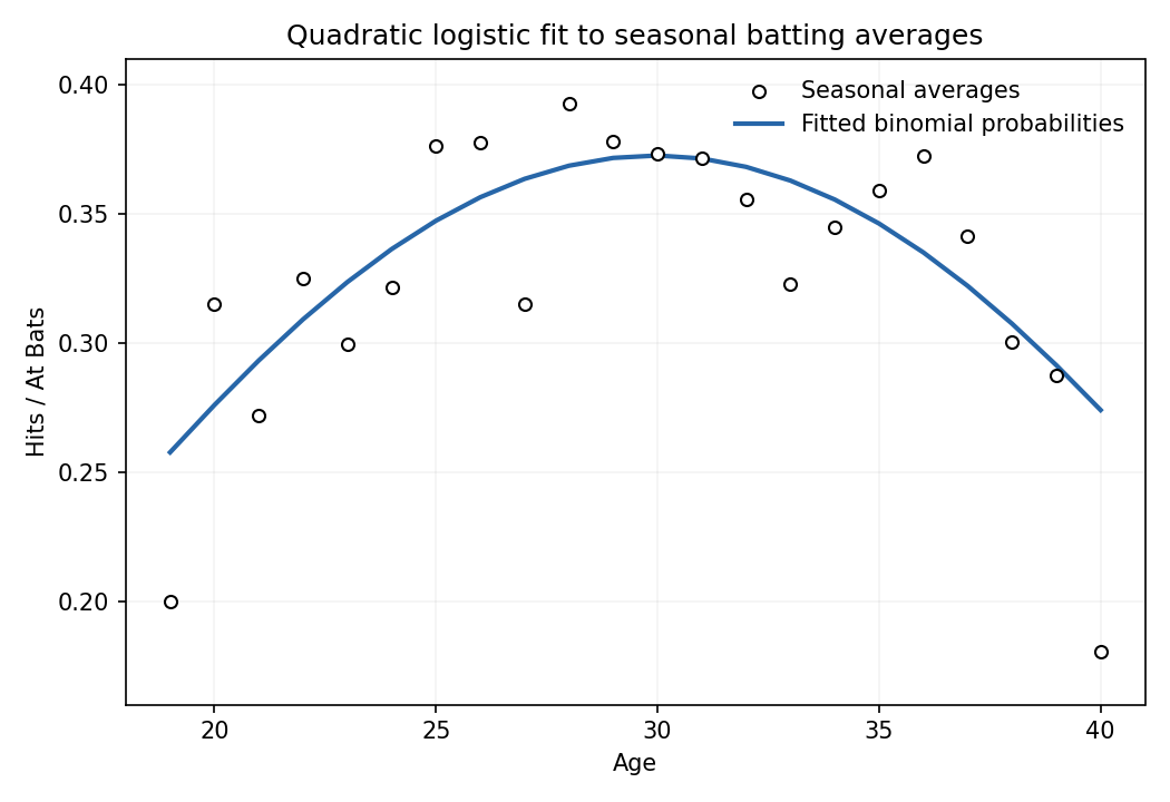
The final commands recover the coefficients, apply the inverse logit $p=(1+e^{-\eta }{)}^{-1}$, plot the observed averages against age, and join the fitted probabilities at the observed ages. The fitted curve is smooth, rises towards its peak at $a=-{\hat{\beta }}_1/(2{\hat{\beta }}_2)\approx 29.95$, then falls. Its maximum is about 0.373; the early and late observed points include markedly lower averages. The plot uses equally sized points even though their binomial precisions differ.