Use the linear dispersive Stokes equation with time variable . Put . Expanding the required local relation givesChoose . Direct differentiation then yieldsThe unwanted coefficient of cancels precisely when . HenceWith these choices, the local relation is exactly for every complex spectral parameter for a linear boundary value problem.
Define the negative-exponential Half-range Fourier transformswhich are holomorphic for . Write and define the finite-time spectral boundary transformsIntegrate the local relation over , . The spatial boundary term at infinity vanishes by decay, and the term at is subtracted. Consequently the half-line linear dispersive Stokes global relation isFourier inversion on the real axis gives an initial-data integral plus an integral of . To put the boundary term on a complex contour, setFor , , so is the connected upper domain , . Orient with this domain on the left: from upper-left infinity down to , along the real segment to , and then to upper-right infinity.
The finite-time spectral boundary transforms are entire functions. In the upper regions outside , where , their time-integrated factors satisfy for . Together with , this permits contour deformation of the two remaining real-axis pieces to the curved boundary of . The resulting representation isThe contour orientation accounts for the plus sign in this convention. This formula still contains the two unknown derivative traces through .
The dispersion relation has two additional arguments with the same value. Indeed,Thus use the cubic Stokes dispersion symmetryBoth roots are in the lower half-plane for . At , , their imaginary parts are . A root cannot cross the real axis in , since a real root would make . Continuity therefore proves the claim throughout this connected domain. The branch points are outside ; interchanging the two root labels does not change the formula below.
Evaluate the global relation at each , where its analyticity requirement holds:The left side is linear in . Interpolate it to the argument with weightsThey satisfy and . HenceFor the last coefficient, useadding and subtracting the interpolated gives .
The remaining solution-transform contribution is . Its integrand is holomorphic in : the transformed arguments remain in the lower half-plane. The weights are bounded at infinity, and supplies decay on the upper closing arc for . The Cauchy integral theorem therefore makes this integral zero. PutThe Dirichlet spectral representation for the linear dispersive Stokes equation is nowAll quantities in this expression are transforms of the prescribed initial and boundary values. Neither derivative trace remains.
Fix . In the representation from (c), the finite-horizon extension of a boundary transform allows to be replaced by . To see this directly, their difference contributesIt has an holomorphic integrand inside ; there , and the factors and allow the contour to be closed. Its integral is zero for . This replacement puts the observation-time dependence entirely in .
Every such exponential satisfies the linear dispersive Stokes equation, becauseConsequently the representation satisfies the partial differential equation. The stipulated smoothness and decay justify the differentiated oscillatory integrals, or equivalently their regularized limits. The fixed horizon is useful here: no artificial source term arises from differentiating the endpoint of a time transform.
At , use the original version. The integral vanishes after closing inside , since is holomorphic there and . Fourier inversion of the initial half-line transform therefore givesFor the boundary trace use the fixed-horizon version, with . First consider the initial-data terms at . Differentiating givesThus changing variables separately in the two pieces of the integral giveswhere goes from lower-left infinity to , across to , and then to lower-right infinity along . For completeness, on the upper-right curved edge one root maps onto the real ray and the other onto the lower-right curved edge. On the upper-left edge the corresponding images are and the lower-left edge. The middle segment maps to the remaining real intervals and . These real images cancel the outer pieces of the original real-axis integral, leaving exactly with the stated orientation.
This contour bounds the lower-central region , . The spatial transform is holomorphic there and decays on its closing arcs for . Its integral is therefore zero by the Cauchy integral theorem. The initial-data part of the boundary trace vanishes.
In the remaining boundary integral, use . Along the oriented , traverses the imaginary axis once from to . On its real segment, the imaginary part runs from to ; the two curved edges supply the complementary intervals. It follows thatThe last equality is ordinary temporal Fourier inversion, after . Because is strictly inside it gives the full value, not a truncated-transform endpoint half-value. ThusCompatibility makes the two traces agree at the corner. Spatial decay follows from the upper-contour exponential and nonstationary oscillatory estimates on the real integral as , under the assumed data decay.
The decaying smooth solution is also unique. For a zero-data difference , integration by parts in the linear dispersive Stokes equation givesusing and decay at infinity. The initial norm is zero, so . This completes verification of the initial value, boundary value and governing equation.
Use the Wirtinger derivatives and . The Laplace equation gives , so writewhere is holomorphic in the first quadrant and is holomorphic in the fourth quadrant. They are independent functions: the data may be complex, so a complex-conjugation relation between them cannot be assumed.
Let , where . The oblique derivative boundary conditions becomeThe hinted complementary traces would giveHere is a function of on the horizontal side; the printed range in that hint is a variable typo. We shall eliminate the same unknown traces by reflection of the holomorphic derivatives.
The polygonal ray formula can first be viewed as the Cauchy integral formula. For an oriented edge point , choose its spectral ray so that decays for interior . ThenInterchanging the edge and ray integrals in the supplied formula gives , with counterclockwise edge orientation. Thus a quadrant limit of that formula can be evaluated by the corresponding holomorphic boundary jumps, provided the additional arcs at infinity and at the corner give no contribution.
Define an holomorphic function separately in the four quadrants byThe angle condition gives . It makes the reflected definitions consistent, with parity . On each axis oriented outward from zero, let . The two known boundary equations give all four jumps:For example the vertical equation gives ; reversing the jump order on the upward axis accounts for its displayed sign. The horizontal equation similarly supplies the positive real-axis jump, and reflection supplies the other two.
Apply the Cauchy integral formula in the four quadrants and combine their common edges. The edge contributions are exactly the known jumps of this scalar Riemann-Hilbert problem. If the corner and large-arc integrals vanish, the representation in the first quadrant isThis is the rational-angle oblique derivative problem on a quadrant representation, with all unknown traces removed. The Cauchy integrals have precisely the displayed jumps by the Sokhotski–Plemelj formula. Their reflection parity then reconstructs from the fourth-quadrant value of , so the two original boundary equations hold. Integrating and gives a harmonic function up to an additive constant.
To put the answer back on the spectral rays of the question, defineUse , , and the same identities with replaced by and the ray . The spectral representation isAll transforms used on these rays are ordinary boundary values of convergent half-line transforms. For with , the real-ray integrand decays through and the imaginary-ray integrand through .
There is an admissibility qualification in passing from a bounded polygon to this unbounded quadrant. Sufficient conditions are at infinity uniformly away from the axes, with the corresponding large-arc integral tending to zero, and uniformly on small corner arcs. The latter allows logarithmic gradient singularities but excludes a pole with nonzero corner contribution. Smooth decaying data alone, as printed, do not impose these conditions on .
For a concrete homogeneous corner ambiguity in a quadrant Laplace problem, with and zero data, satisfies both prescribed tangential derivative conditions but has , while the displayed particular representation is zero. With , the zero-data solution has : it decays at infinity but has an excluded corner pole. Thus no unique representation of every unrestricted solution follows from the printed data alone. Without the arc conditions, one must add a homogeneous holomorphic term to the displayed , with reflected parity ; permitted corner singularities are included if the admissible class allows them. With the stated decay and corner conditions that term vanishes, giving the boxed formulas. This identifies the missing solution-class conditions without assuming real-valued data.
Take the negative-exponential Half-range Fourier transform and setThe advection-diffusion equation has the local relation with flux . Integration over the half-line gives the half-line drift global relationFor the upper decay domainwrite . It is the region above , in particular above . Its boundary is oriented from upper-left infinity through to upper-right infinity, with the domain on the left. Fourier inversion and deformation of the boundary terms giveUse the dispersion symmetry elimination of a boundary trace . It preserves and maps into the lower half-plane. Because , the global relation at impliesThe last term contributes an holomorphic upper-domain integral multiplied by , so it vanishes upon closing the contour for . The solution representation with only known data is consequentlyFor the boundary value , direct integration givesThis quotient is an entire function of when its apparent singularities at are filled by their limits. Those points are not genuine forcing poles of the finite-time transform.
To obtain an exponentially decaying spectral integrand, choose and the exponential-decay contour for half-line drift diffusionDeform to . No pole is crossed: the initial-data denominator in that boundary integral has its only pole at , which lies below since . The apparent singularities of the forcing transform are removable. In the swept outer sectors, has the appropriate bounded growth for the deformation. The contour formula becomesEvaluate the second quotient as a removable expression at , rather than splitting it into artificial residue terms. On either ray,Since , the transient factors have Gaussian decay as . The nontransient forcing term is and thus also decays exponentially for every . The real-axis integral has the Gaussian factor . These estimates provide the requested improvement over integration along .
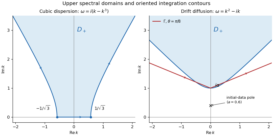
Upper cubic-dispersion contour and exponentially decaying drift-diffusion contour, with their orientations
. Details. 
The first panel shows the cubic domain from Question 1. The second uses and ; its marked initial-data pole corresponds to and lies below both boundary contours.
An independent real-kernel form also makes the initial and boundary traces explicit. Apply the Dirichlet gauge transform for constant drift, , and then multiply by to obtain the heat equation. The odd-reflected heat kernel for initial data and its Dirichlet boundary-forcing heat-kernel formula yieldThe first kernel tends to the initial delta kernel on as and vanishes at . For the second kernel, the substitution gives the unit-mass approximate boundary delta as , so its trace is ; it vanishes initially for fixed . Differentiating the kernels for verifies the advection-diffusion equation. The integrals converge for every positive , even when the exponentially weighted initial datum grows, because the spatial Gaussian controls that growth. Thus this gives the same decaying solution without introducing an additional restriction on .
For a general decaying initial datum, an unweighted Fourier sine transform does not directly diagonalize the drift operator. DefineTwo integrations by parts for and one for giveThe cosine transform remains unknown, so this is not a closed sine-transform evolution. In contrast, the weighted sine transform for half-line drift diffusion of is closed:When the weighted initial transform exists, Fourier sine inversion gives . This method requires suitable decay of , not merely decay of . For the exponential datum it is an ordinary integrable sine transform only when . At one would need a generalized or regularized transform instead; the contour and real-kernel formulas above already work without that restriction. Therefore the ordinary sine transform of is not a closed solution method; a weighted sine transform works under the stated extra weighted-decay condition.
Articles by others on the same topic
There are currently no matching articles.