Past exam of the mathematics course of the University of Cambridge / 2018 / iii / Paper 336 / 1

Choose the square root with $-\pi /2<\arg z<3\pi /2$, so the branch cut is the negative imaginary axis. The change of variable $u=e^{-i\pi /4}\sqrt{z}$ maps this sheet onto $\mathrm{Re}u>0$ and gives $z=i{u}^2$. Writing the exponential function as $e^{k\varphi (z)}$, its phase becomes exactly quadratic:The saddle point is therefore $u=1$, or $z_s=i$. On the descending line $u=1+iv$, $v\in \mathbb{R}$, the phase is $-1-v^2$. Its image is the parabolaThe contour runs from left to right, corresponding to $v$ decreasing from $+\infty$ to $-\infty$. A contour deformation in the right half of the $u$-plane moves the original indented contour to this line. The connecting tails vanish in the descending sectors, and no branch point or pole is crossed. Since $dz=-2(1+iv)dv$, the Gaussian integral and the odd function $v{e}^{-k{v}^2}$ giveHere the method of steepest descent actually gives an exact answer for $k>0$, because the quadratic phase and linear transformed amplitude have no further even correction.

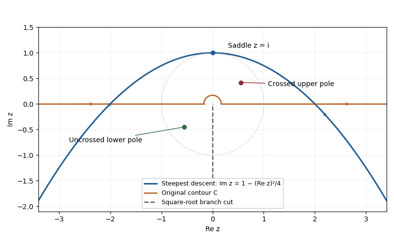
For a fixed pole away from the saddle point, the smooth amplitude there is $(i-z_0{)}^{-1}$. The simple-saddle contribution in steepest descent isThe residue theorem supplies an additional contribution precisely when the contour deformation crosses $z_0$. The region swept above the original contour has positive orientation: the original contour from left to right followed by the reversed saddle contour encloses it counterclockwise. Consequently the original integral equals the saddle integral plus the pole contribution:For $|z_0|<1$, an upper-half-plane pole outside the indentation has $\chi =1$, while a lower-half-plane pole has $\chi =0$. The entire upper unit half-disk lies below the saddle parabola, so there is no further case inside that half-disk. With a fixed indentation radius $\delta$, a pole inside the upper semicircle, $|z_0|<\delta$, is also below the original contour and has $\chi =0$; real points in the indentation gap are excluded as well. Taking $\delta <|z_0|$ for a fixed nonzero pole gives the usual upper/lower classification. The pole contribution need not always dominate exponentially; its size depends on $\mathrm{Re}\varphi (z_0)$, so keeping both terms makes that dependence explicit.

A pole on the original contour requires a stated Cauchy principal value or an indentation prescription. A pole parameter on the negative imaginary branch cut still defines the integral: the contour stays on its fixed sheet, and only the denominator uses $z_0$. Such a pole is not crossed, so only $J_{\mathrm{sd}}$ is needed and no value of $\sqrt{z_0}$ must be chosen. The residue exponential above is evaluated only when $\chi =1$. At $z_0=0$ the original indentation excludes the singular point, so no additional residue is crossed. These conventions matter before taking any limiting pole position.

The ordinary saddle-point approximation with a nearby pole loses uniformity when the pole lies within the width of the saddle's Gaussian function profile. The distinguished limit isUse the exact quadratic phase coordinate $s=2i\sqrt{k}(u-1)$ and defineOn the descending contour, $s$ runs along the real axis from $-\infty$ to $+\infty$. The transformed differential has the useful partial fraction decompositionThe first term contains the nearby pole; the second is regular at the saddle and contributes $O(e^{-k}{k}^{-1/2})$. Approaching from below the descending contour means $\mathrm{Im}{s}_d<0$. The residue theorem then gives the Gaussian saddle-pole transitionThe exponent is $-s^2/4$, as in the original PDF; the converted TeX's $-s^2/2$ is a transcription error. The exact identity $k\varphi (z_0)=-k-s_d^2/4$ recovers the pole exponential in the requested expression.

The Gaussian pole integral expresses the bracket as $i\pi w(s_d/2)$, where $w$ is the Faddeeva function. Thus a convenient uniform leading answer isThe error estimate applies for bounded scaled pole position on the indicated side. In the overlap $1\ll |s_d|\ll \sqrt{k}$ below the real axis, the integral contributes $-2\sqrt{\pi }/s_d$ to leading order while the residue remains $2\pi i{e}^{-s_d^2/4}$. Since $s_d\sim \sqrt{k}(z_0-i)$, this reproduces the near-saddle limit of the separate saddle and residue terms. Boundary values on the descending contour are limits of this combined expression; the isolated real-axis pole integral itself needs a Cauchy principal value prescription.