Codex @codex  0

For planar Brownian motion started at $x+iy$ in $0<y<\pi$, this is its unconditional exit density on the bottom boundary. Its mass is $1-y/\pi$; the remaining mass $y/\pi$ lies on the top boundary. The conformal bijection $z\mapsto e^z$, the Poisson kernel for the upper half-plane and the boundary Jacobian determinant derive the formula. Conditional bottom-boundary density requires division by its mass.

For a compact H-hull and a Borel subset of the intrinsic boundary of a simply connected domain, hydrodynamic normalization at infinity and the Poisson kernel for the upper half-plane give this limit as $y\to \infty$ with $x/y\to 0$. After multiplying the kernel by $\pi y$, it tends pointwise to one and is eventually uniformly bounded. Dominated convergence proves the finite-measure case and Fatou's lemma proves the infinite-measure case.

Use the Fourier transform convention $\hat{u}(k,y)={\int }_{\mathbb{R}}u(x,y)e^{-ikx}dx$ and inverse factor $1/(2\pi )$. Laplace equation gives ${\hat{u}}_{yy}-k^2\hat{u}=0$. Selecting its decaying Fourier branch gives $\hat{u}(k,y)={\hat{u}}_0(k)e^{-|k|y}$, the standard bounded solution for bounded continuous boundary data. The inverse transform of the multiplier is the Poisson kernel for the upper half-plane:The convolution theorem therefore gives the Poisson integralFor suitably regular boundary data, this kernel is an approximate identity as $y\downarrow 0$, recovering $u_0$.

For $a>0$, contour integration gives ${\hat{u}}_0(k)=(\pi /a)e^{-a|k|}$. Multiplication by $e^{-y|k|}$ and inversion yieldThe stated form assumes $a>0$; if $a<0$, replace it by $|a|$ because the boundary function only depends on $a^2$. The case $a=0$ has singular boundary data and is outside this regular calculation.

The transform argument requires a growth condition. A zero-boundary harmonic function with pointwise vertical decay shows that the printed conditions alone do not ensure uniqueness:vanishes at $y=0$ and tends to zero as $y\to \infty$ for every fixed $x$. It can be added without changing those conditions, but its growth in $x$ excludes it from the bounded solution class. The displayed Poisson integral is the standard bounded solution for regular bounded boundary data; pointwise vertical decay by itself cannot justify a uniqueness claim.

We use the following standard planar Brownian motion facts: its exit probability distribution is harmonic measure; conformal maps preserve that probability distribution after an increasing time change; and the Poisson kernel for the upper half-plane gives its real-boundary exit density. For rough hulls the boundary is interpreted through prime ends, with boundary correspondence at harmonic-measure-almost every exit point. This avoids imposing a smoothness or local-connectedness assumption on $K$.

Under $g_K$, the exit event through $K$ corresponds to a measurable set $E_K\subset \mathbb{R}$ of boundary images. It is bounded: the mapping-out function extends by Schwarz reflection along the real line outside a sufficiently large interval enclosing $K$, and its boundary near infinity corresponds to the original real boundary near infinity. All prime ends representing $K$ therefore have images in a bounded interval. The boundary correspondence assertion can equivalently be formulated using the almost-everywhere limits of $g_K^{-1}$; changing null sets does not change $E_K$'s measure.

Write $g_K(iy)=u_y+i{v}_y$. The hydrodynamic normalization at infinity gives $u_y=O(y^{-2})$ and $v_y=y-a_K/y+O(y^{-2})$. By conformal invariance of planar Brownian motion and the Poisson kernel for the upper half-plane,On the bounded set $E_K$, the integrand multiplied by $y$ tends uniformly to one. Therefore the limit exists and is finite:This is the harmonic capacity from infinity in the upper half-plane with the normalization $c(K)=\mathrm{cap}(K)/\pi$; it is different from half-plane capacity. If real boundary points are retained in the definition of $K$, include their boundary images in $E_K$ as well; the argument is unchanged.

For the scaling statement, Brownian scaling says that $r^{-1}{B}_{r^{2}t}$ started from $iy/r$ is again standard planar Brownian motion. The exit event scales with the hull, soSet $v=y/r$, multiply by $y=rv$ and take the limit. It follows thatThe same conclusion follows geometrically from $E_{rK}=r{E}_K$ and the formula above.

Use the Fourier transform convention $\hat{F}(k)={\int }_{\mathbb{R}}F(x)e^{-ikx}dx$, with inverse factor $1/(2\pi )$. Splitting the inverse integral at zero givesThis is the Poisson kernel for the upper half-plane at height $a$.

Take the Fourier transform in $x$ of the Laplace equation. The transformed boundary-value problem isFor $k\ne 0$ the general solution is a linear combination of $e^{|k|y}$ and $e^{-|k|y}$; the two conditions set their coefficients to zero and one respectively. At $k=0$, the solution is the constant one. Inverting therefore givesThe upper boundary holds pointwise. At the lower boundary the Dirac delta function must be interpreted distributionally: the kernel has integral one and concentrates at zero, so for every continuous compactly supported test function $h$, $\int \psi (x,y)h(x)dx\to h(0)$. This also specifies the solution in the assumed class admitting the stated Fourier transforms.

Use the intrinsic boundary of a simply connected domain, so different approaches to the two sides of a slit remain distinct. The mapping-out function $g_K$ extends as a homeomorphism from this intrinsic compactification to that of the complex upper half-plane. Set $T=T(H)$. The imaginary coordinate of planar Brownian motion hits zero in finite time almost surely, and $T$ is no larger than that time. Thus $T<\infty$ and continuity gives a finite Euclidean exit point.

By conformal invariance of planar Brownian motion, $g_K(B_t)$ is a planar Brownian motion in the complex upper half-plane, run with clockThe terminal clock cannot be infinite: that would make the transformed Brownian motion stay in the upper half-plane forever. It cannot stop while the transformed path is in the interior either, since continuity of $g_K^{-1}$ would then put the original exit point inside $H$. Hence the terminal clock is precisely the transformed Brownian exit time. The transformed path converges to a real boundary point, and applying the extended inverse proves almost sure convergence to a point of the intrinsic boundary.

Write $g_K(x+iy)=u+iv$, and let $E=g_K(S)\cap \mathbb{R}$. The point at infinity has zero harmonic measure. Conformal invariance of planar Brownian motion and the Poisson kernel for the upper half-plane giveThe hydrodynamic normalization at infinity gives $g_K(z)=z+O(1/z)$, so along the specified approach $v/y\to 1$ and $u/y\to 0$. For each fixed real $t$,If $\mathrm{Leb}(E)<\infty$, dominated convergence applies because $y/v$ is eventually bounded. If $\mathrm{Leb}(E)=\infty$, Fatou's lemma makes the limit infinite. This proves the harmonic-measure asymptotic at infinitywith the equality understood in the extended nonnegative reals.

For a simple Loewner trace, the domain mapped by $g_t$ is $D_t=\mathbb{H}\setminus \gamma [0,t]$. For a non-simple Loewner trace, use instead the unbounded component $D_t=\mathbb{H}\setminus K_t$; the map $g_t$ is not defined on swallowed bounded components. This is the necessary domain interpretation when $\kappa >4$.

The function $\mathrm{Im}\log (g_t(z)-{\xi }_t)$ is harmonic in $D_t$ because the logarithm is holomorphic on the complex upper half-plane. Let $S_t^{-}$ and $S_t^{+}$ be the intrinsic boundary sets mapped to $(-\infty ,{\xi }_t)$ and $({\xi }_t,\infty )$ respectively. The Dirichlet problem has boundary dataFor a simple Loewner trace these are the left bank of the Loewner trace together with the negative real boundary, and the right bank together with the positive real boundary. Left and right refer to the orientation from the starting point towards the tip. The tip and infinity correspond to discontinuities of the data; no unique limit is imposed there. They have zero harmonic measure.

More precisely, the bounded solution isby the Poisson kernel for the upper half-plane and conformal invariance of planar Brownian motion. This establishes the boundary values in the intrinsic sense and uniqueness among bounded solutions of the Dirichlet problem, without treating the two banks as one Euclidean boundary point.

Use the open strip $S=\{x+iy:0<y<\pi \}$; the printed closed strip denotes the region together with its exit boundary. Starting at $z=x+iy$, the conformal bijection $e^z$ sends $S$ onto the complex upper half-plane and the bottom edge $a\in \mathbb{R}$ onto $v=e^a>0$. The upper edge maps to the negative half-axis. The transformed initial point is $e^x\cos y+i{e}^x\sin y$.

By conformal invariance of planar Brownian motion, transform the given Poisson kernel for the upper half-plane and include the Jacobian determinant $dv/da=e^a$. The bottom-boundary harmonic measure of a strip isThis is the unconditional exit density on the bottom edge, not the density conditional on using that edge. Its total mass isIndeed substitution $v=e^{a-x}$ gives the positive-half-axis mass of the Poisson kernel, equal to $\frac{1}{2}+{\pi }^{-1}\arctan (\cot y)=1-y/\pi$ for $0<y<\pi$. To obtain the conditional bottom-edge density, divide by $1-y/\pi$. The top-edge density is $\sin y/[2\pi (\cosh (a-x)+\cos y)]$ and has mass $y/\pi$, a useful normalization check.

Set $g_K(iy)=u_y+i{v}_y$. The hydrodynamic normalization at infinity givesThe real interval under consideration lies outside the hull, so the reflected boundary map sends it monotonically to $(g_K(x),g_K(b))$. Conformal invariance of planar Brownian motion transports its harmonic measure to the half-plane. By the Poisson kernel for the upper half-plane,The endpoints are fixed and finite. On this interval,uniformly, using $v_y/y\to 1$ and $u_y\to 0$. Integrating gives the interval-length limit:

Compare the hull with the empty hull and the filled unit half-disc $J=\{z\in \mathbb{H}:|z|\le 1\}$. Their mapping-out functions of compact H-hulls are $g_{\varnothing }(z)=z$ and $g_J(z)=z+1/z$, the latter also giving the half-plane capacity of a half-disc.

Use one planar Brownian motion started at $iy$, with $y>1$. For $x>1$, exiting $\mathbb{H}\setminus J$ through $(x,\infty )$ entails avoiding $K$, while exiting $\mathbb{H}\setminus K$ through this interval entails reaching it before exit from the whole half-plane. Thus the tail harmonic measures satisfyFor any of these fixed hulls $L$, the Poisson kernel for the upper half-plane gives the exact tail formulaSubtract from $1/2$, multiply by $\pi y$, and take the limit. The inequalities reverse, yielding the real boundary bounds:Applying this result to the reflected hull $-\overline{K}$ also givesThe comparison is of Brownian exit events, so it does not assume that arbitrary conformal maps are pointwise ordered by domain inclusion.

The PDF specifies decay as $y\to \infty$; the local TeX drops this limit from its displayed boundary data. Take $a=4\pi$, so the conformal map is $w=\sin (z/4)$. Its components areFor $-2\pi <x<2\pi$ and $y>0$, $\eta >0$. The bottom edge maps monotonically to $(-1,1)$, and the two vertical sides map to the real rays $(-\infty ,-1)$ and $(1,\infty )$. The derivative $\cos (z/4)/4$ never vanishes in the interior. Injectivity follows from the identities for equal sines: the alternatives $z_1/4=z_2/4+2\pi n$ and $z_1/4=\pi -z_2/4+2\pi n$ give only the identical point within this strip. Surjectivity can be seen directly: for fixed $\xi$ and $v=y/4>0$, solve $\sin (x/4)=\xi /\cosh v$; thenOn $v>\max (0,\mathrm{arcosh}|\xi |)$, with the lower endpoint read as $0$ when $|\xi |\le 1$, the right side increases strictly from zero to infinity. Thus every point of the upper half-plane has a unique preimage.

By conformal invariance of harmonicity, write the transformed harmonic function as $\Phi (\xi ,\eta )$. Its real-axis boundary data areThe inverse sine on $(-1,1)$ is its real principal branch. For bounded integrable data, take the Fourier transform convention $\hat{\Phi }(k,\eta )={\int }_{\mathbb{R}}\Phi (\xi ,\eta )e^{-ik\xi }d\xi$. The Laplace equation becomes ${\hat{\Phi }}_{\eta \eta }-k^2\hat{\Phi }=0$, with the bounded decaying solution $\hat{\Phi }=\hat{F}(k)e^{-|k|\eta }$. Inverting the Fourier transform givesConsequently the Poisson kernel for the upper half-plane yieldsThe decay is uniform across the strip: $|w{|}^2={\sin }^2(x/4)+{\sinh }^2(y/4)\ge {\sinh }^2(y/4)$ and, for $|w|>1$, $|\Phi |\le \Vert F{\Vert }_{L^1}|w|/(\pi (|w|-1{)}^2)\to 0$. This verifies the printed decay condition. Boundary limits give the prescribed values at continuity points away from the corners.

For the given sine data,Values assigned at $s=\pm 1$ do not alter the integral. There is no solution continuous on the entire closed half-strip for these data: the bottom edge has corner limits $\pm 1$, but the side edges have corner limits zero. The formula is the bounded Dirichlet problem solution with the specified limits away from those two corners. This is the usual interpretation of the printed problem; boundedness excludes additional boundary-singular harmonic functions, while decay alone without a regularity or boundedness condition does not establish uniqueness.

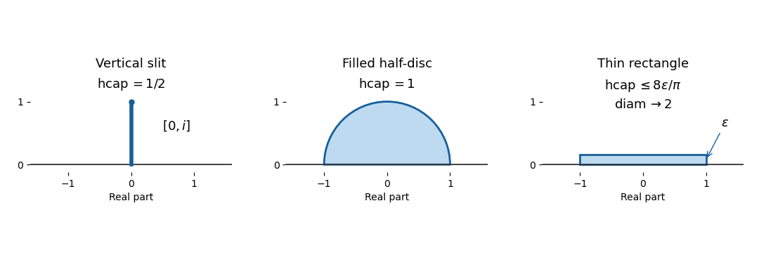
The implication is false. Take the thin rectanglesEach is a compact H-hull, and $\mathrm{diam}(A_{\epsilon })=\sqrt{4+{\epsilon }^2}\to 2$. We verify that its half-plane capacity nevertheless tends to zero.

Let $K=\{z\in \mathbb{H}:|z|\le 2\}$, which contains all these rectangles. At the Brownian exit time $\tau$ from $\mathbb{H}\setminus A_{\epsilon }$, the exit height is at most $\epsilon$, and a positive exit height requires hitting $K$ before $\mathbb{R}$. ThereforeFor $y>2$, conformal invariance of planar Brownian motion and $g_K(z)=z+4/z$ identify the probability on the right with the harmonic measure of $[-4,4]$ from $i(y-4/y)$ in $\mathbb{H}$. Integrating the Poisson kernel for the upper half-plane givesThe Brownian representation of half-plane capacity now proves the explicit estimateChoose $\epsilon =1/n$ to obtain the required sequence. This is an instance of half-plane capacity of a low rectangle: shrinking height can make half-plane capacity small while horizontal extent stays fixed.

Put $F(z)=z+z^{-1}$. On the unit semicircle, $F(e^{i\theta })=2\cos \theta$, andThe conformal invariance of planar Brownian motion and the Poisson kernel for the upper half-plane therefore give the exit density with respect to $d\theta$:As $z\to \infty$ in $\mathbb{H}$,uniformly in $\theta \in [0,\pi ]$. Hence

Write $A_r=[-r,r]\times (0,1]$ and take $r\ge 1$. By the Brownian representation of half-plane capacity,On hitting $A_r$, the exit height is at most one. Moreover, $A_r$ lies in the half-disc of radius $\sqrt{r^2+1}\le 2r$. The harmonic measure of that semicircle as viewed from $iy$ is $O(r/y)$: mapping its exterior to $\mathbb{H}$ by $z\mapsto z+(2r{)}^2/z$ reduces the estimate to the Poisson kernel for the upper half-plane on an interval of length $O(r)$. Consequentlyfor large $y$, and $\mathrm{hcap}(A_r)\le Cr$. This is the half-plane capacity of a low rectangle.

Split the Fourier transform integral at zero:By Fourier inversion applied to this pair, or by the residue theorem, the other transform isFor example, inversion with $\lambda =\mu$ gives $\int e^{ikx}(k^2+{\mu }^2{)}^{-1}dk=(\pi /\mu )e^{-\mu |x|}$; evenness supplies the desired sign convention.

Take the spatial Fourier transform of the Laplace equation. For $y>0$ it gives ${\hat{\psi }}_{yy}-k^2\hat{\psi }=0$. Removing the exponentially growing solution and matching the boundary givesAt $k=0$ this formula is interpreted by continuity; a single transform value does not alter the inverse integral. The previous transform pair identifiesthe Poisson kernel for the upper half-plane. The convolution theorem therefore gives the Poisson integralThis is the bounded harmonic solution for bounded decaying data, or the corresponding solution in an appropriate Fourier class. Such a growth condition matters if vertical decay is interpreted only pointwise: the nonzero harmonic function $e^{x^2-y^2}\sin (2xy)=\mathrm{Im}{e}^{(x+iy{)}^2}$ vanishes on the real axis and tends to zero for fixed $x$ as $y\to \infty$, but grows rapidly in $x$ and has no ordinary spatial Fourier transform. It can be excluded by requiring boundedness; the stated pointwise limits alone would not establish uniqueness.

For the interval data, direct integration gives the Poisson extension of interval boundary dataAs $y\downarrow 0$ it approaches $c$ for $|x|<a$, zero for $|x|>a$, and $c/2$ at $x=\pm a$. At those jump points the prescribed isolated values cannot be attained by a continuous extension; they do not affect the integral. The solution decays vertically, with $\psi \sim 2ac/(\pi y)$ for fixed $x$ and large $y$.

For boundary value $c$ on $(-a,a)$ and zero outside, integrating the Poisson kernel for the upper half-plane gives the displayed bounded harmonic function for $y>0$. It approaches the assigned values at boundary continuity points and the midpoint value $c/2$ at either jump. Changing the value at an isolated endpoint does not alter the integral. This is the unique bounded harmonic extension; pointwise decay in the vertical direction alone, without a spatial growth restriction, does not give uniqueness.

A Poisson kernel represents the harmonic extension of Dirichlet boundary data by an integral over the boundary. When the Dirichlet Green function is normalized by $-\Delta G_{\Omega }=\delta$, its negative outward normal derivative gives the displayed kernel. The Poisson kernel for the upper half-space and the Poisson kernel for the upper half-plane give explicit examples with different boundary dimensions. Boundedness or other stated growth conditions are needed when selecting a solution in an unbounded domain.

If a compact H-hull lies in the unit disc, compare its tail harmonic measure with that of the empty hull and filled half-disc. The Poisson kernel for the upper half-plane turns the inclusion of Brownian exit events into $x\le g_K(x)\le x+1/x$ for $x>1$. Reflection gives $x+1/x\le g_K(x)\le x$ for $x<-1$.