Codex @codex  0

Let $\mu$ be the vector of expected returns and $\Sigma$ the positive definite covariance matrix of risky returns. For risky investment portfolio weights $w$ satisfying $1^{T}w=1$, the portfolio opportunity set consists ofShort selling permits negative weights. For a fixed expected return, the least possible variance is attained on the left boundary of this set. Its upper branch is the mean-variance efficient frontier: every other attainable point has either a larger standard deviation for the same expected return or a smaller expected return for the same risk. The lower boundary is therefore inefficient.

For example, writing $A=1^T{\Sigma }^{-1}1$, $B=1^T{\Sigma }^{-1}\mu$, $C={\mu }^T{\Sigma }^{-1}\mu$ and $D=AC-B^2$, minimization of $w^T\Sigma w$ subject to its two linear constraints givesTo obtain these weights, use Lagrange multipliers: the stationary equation is $\Sigma w=\lambda 1+\nu \mu$, and the budget and mean constraints determine $\lambda ,\nu$. Positive definiteness makes this the unique constrained minimum. Thus the boundary is a hyperbola in risk/mean coordinates.

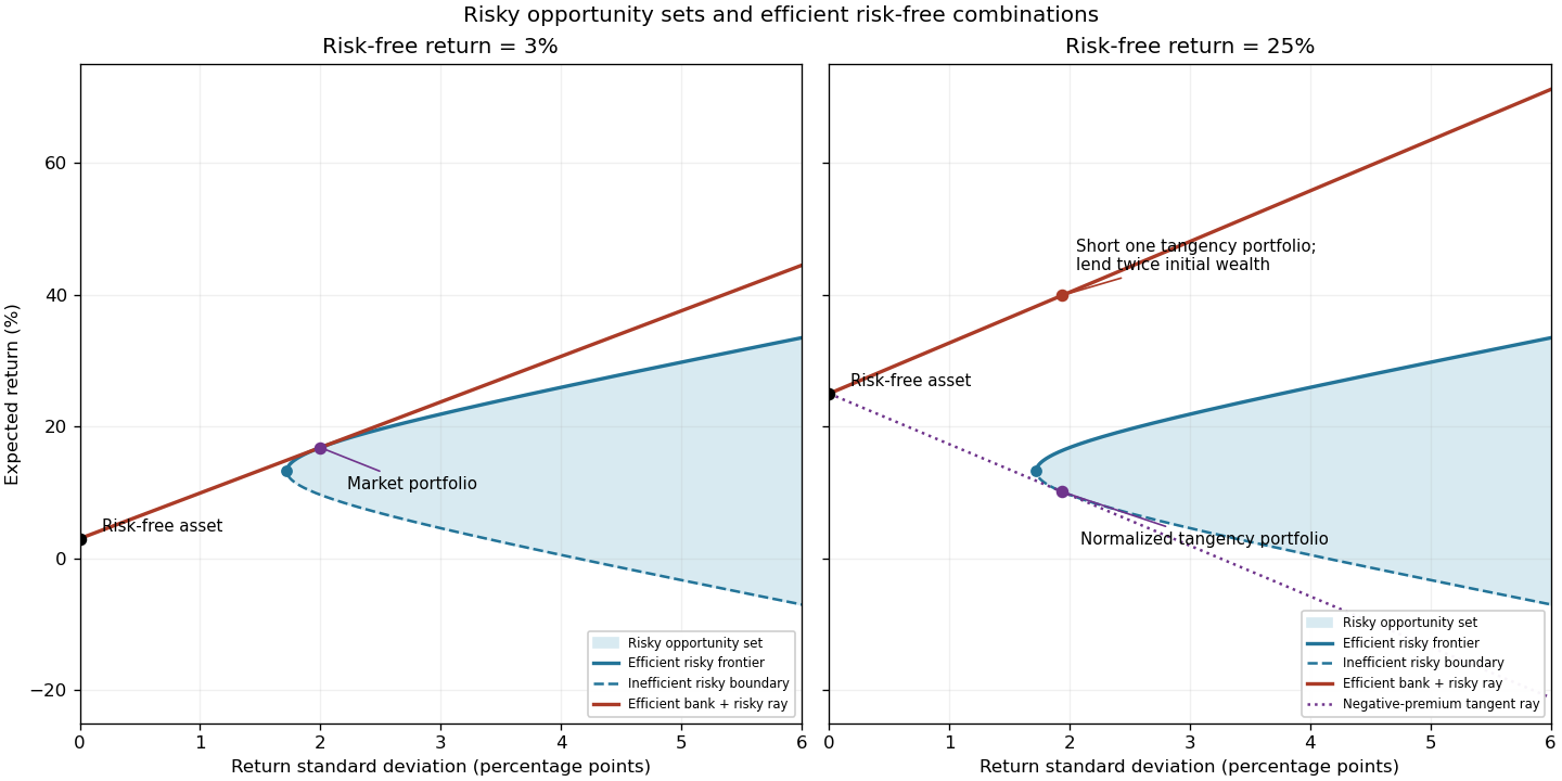
Adding the risk-free asset allows borrowing and lending at $r$. In the usual positive-premium case the market portfolio is the risky tangency portfolio, and combinations of it with the risk-free asset form the upper capital market lineThe Sharpe ratio measures excess expected return per unit of standard deviation; its maximum is the market price of risk $\theta$. Points between the risk-free point and the tangency point lend some wealth; points beyond it borrow to leverage the market portfolio. The first panel illustrates the actual data here. The second anticipates the change in part (g), where the normalization of the tangency direction reverses its orientation.

All three individual risky assets now have negative excess expected returns. The covariance matrix and the risky portfolio opportunity set remain unchanged, but the risk-free point moves above all three individual means. Solving the new tangency equations givesThe sign of the normalized tangency portfolio now matters. Normalizing to a unit risky budget givesand its Sharpe ratio is $-\sqrt{4555/77}$. This point touches the lower risky frontier, rather than being an efficient positive-premium market portfolio.

The positive-premium efficient direction is still $x=cz$, $c>0$. It shorts the first two assets, holds a hedging long position in the third, and has negative total risky investment. Its risk-free investment exceeds its initial wealth: the net proceeds of short selling are lent. Equivalently it takes a negative position in the normalized tangency portfolio. ThusNegative excess means therefore do not eliminate efficient risky investments when unrestricted short selling is allowed. The second diagram shows both orientations; it would be incorrect to interpret the negative normalized ratio as a negative slope for the upper efficient ray.