Covariance matrix ($\Sigma =\mathbb{E}[(X-\mathbb{E}X)(X-\mathbb{E}X{)}^T]$)

For a real random vector $X=(X_1,\dots ,X_p{)}^T$ with finite second moments, its covariance matrix collects all pairwise covariances:The diagonal entries are variances. The covariance matrix is a symmetric matrix and a positive semidefinite matrix, because for every real vector $a$,Thus one matrix describes the variance of every linear combination of the coordinates. It is a positive-definite matrix exactly when no nonzero linear combination is constant almost surely. A deterministic linear relation produces a zero eigenvalue.

For example,has unit coordinate variances, covariance $0.8$, and eigenvalues $1.8$ and $0.2$. Its unit eigenvectors $(1,1{)}^T/\sqrt{2}$ and $(1,-1{)}^T/\sqrt{2}$ describe directions of greatest and least projected variance. For a unit vector $a=(\cos \theta ,\sin \theta {)}^T$, direct multiplication gives $a^T\Sigma a=1+0.8\sin (2\theta )$: the variation in the sum direction is nine times that in the difference direction.

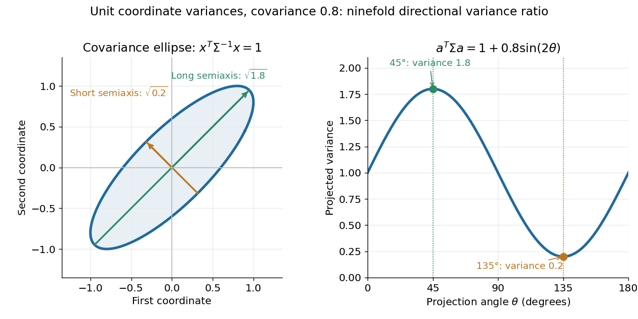
The spectral theorem supplies an orthonormal basis of these directions. This connects covariance matrices to principal component analysis: its leading eigenvector identifies the unit-direction projection with the largest variance. For a linear transformation $A$, the transformed random vector has covariance matrix $A\Sigma A^T$, so uncertainties propagate through a linear model by matrix multiplication.

For a two-dimensional positive-definite covariance matrix $\Sigma$, the centered covariance ellipse is the image of the unit circle under its positive definite square root of a matrix. Equivalently, it satisfies $x^T{\Sigma }^{-1}x=1$. Its semi-major and semi-minor axes have lengths given by the square roots of the larger and smaller eigenvalues, along the corresponding eigenvectors. The ellipse encodes a second-moment geometry; a probability-coverage interpretation needs additional information about the probability distribution and the chosen scale.

For a random vector with covariance $\Sigma$ and positive coordinate variances, let $D=\mathrm{diag}(\Sigma )$. Its correlation matrix is the covariance of $D^{-1/2}(X-\mathbb{E}X)$, so it is positive semidefinite with unit diagonal. Each entry is the correlation of the corresponding pair of variables. In particular $\mathrm{tr}(C)=p$, explaining why an eigenvalue in correlation-based principal component analysis represents that eigenvalue divided by $p$ of the total variance. The empirical version is the sample correlation matrix.

This unit-variance covariance matrix has eigenvalue $1+(p-1)r$ on the constant-vector direction and eigenvalue $1-r$ on its orthogonal complement. It is positive semidefinite exactly when $-1/(p-1)\le r\le 1$. For positive $r$, the first population principal component is the normalized sum of the centered variables.

For a positive-definite covariance matrix, this is Euclidean distance after whitening. It accounts for both scales and correlations and is invariant under consistent nonsingular linear changes of coordinates. Estimating the covariance can be unstable with small samples, and a singular covariance requires restricting to a nonsingular subspace rather than claiming an ordinary metric on the full space.

A compound-symmetry covariance matrix has a common diagonal entry and a common off-diagonal entry: $\Sigma =aI+cJ$. For a group of size $k$, its within-group eigenvalue is $a$ and its constant-direction eigenvalue is $a+kc$. Thus $a\ge 0$ and $a+kc\ge 0$ characterize positive semidefiniteness. When $c\ge 0$, an independent shared random intercept plus individual noise realizes this covariance. A group mean has variance $c+a/k$; a difference of two disjoint subgroup means within the same group cancels $c$.

For a unit vector $u$ and $\theta >0$, a rank-one covariance spike is the covariance matrix $I+\theta u{u}^{\top }$. Its eigenvalue is $1+\theta$ in the direction $u$ and one on the orthogonal complement. It arises by adding an independent scalar normal distribution signal $Yu$ to a standard Gaussian random vector.

The sample mean and covariance estimate the first two moments of a random vector from repeated observations.

The uncentered empirical second-moment matrix averages the outer products of the observations. Its expected value is $\mathrm{Cov}(X)+\mathbb{E}[X]\mathbb{E}[X{]}^{\top }$. It is an unbiased estimator of the covariance matrix when the population expected value is known to be zero. It differs from a sample covariance matrix centered at the sample mean.

For observations $X_1,\dots ,X_n$, the sample mean is $\overline{X}=n^{-1}{\sum }_{i=1}^n{X}_i$.

For independent samples of sizes $n,m$ from populations with means ${\mu }_X,{\mu }_Y$ and finite variances ${\sigma }_X^2,{\sigma }_Y^2$, the difference of their sample means has expected value ${\mu }_X-{\mu }_Y$ and variance ${\sigma }_X^2/n+{\sigma }_Y^2/m$. This uses independence between and within the samples. With dependent samples, a covariance term is required instead.

Partition a sample into two disjoint groups $A,B$ with fixed positive sizes $n_A,n_B$, and let $w=n_A/(n_A+n_B)$. The overall sample mean is the weighted meanSubtracting gives the displayed identity. The subgroup and overall sample means share observations, so they are not independent. If the two disjoint groups are sampled independently, thenThus treating the subgroup and the combined sample as two independent samples uses the wrong standard error. Equality of the subgroup and overall population means is equivalent to equality of subgroup and complement means when both groups have positive weight, but the sampling distribution must respect the shared observations.

For independent and identically distributed observations with finite positive variance, the central limit theorem, consistency of the sample variance and Slutsky's theorem give $T_n\stackrel{d}{\to }N(0,1)$. Under an independent normal distribution sample it instead has the exact finite-sample Student t-distribution with $n-1$ degrees of freedom, as described by the studentized normal sample mean. The asymptotic statement does not require normal individual observations.

For observations $x_1,\dots ,x_n$, the sample covariance matrix is $n^{-1}{\sum }_i(x_i-\bar{x})(x_i-\bar{x}{)}^T$, or the same sum divided by $n-1$ under the unbiased convention.

If $H=I_n-11^T/n$ and $S=X^{T}HX/n$, then $\mathrm{rank}S=\mathrm{rank}(HX)\le \min (p,n-1)$. In particular full column rank of raw $X$ does not ensure a nonsingular centered sample covariance matrix. When $S$ is singular, its Gaussian precision profile likelihood has no finite maximizer: increase precision along a nonzero null vector.

For paired scalar observations $(x_i,y_i)$, their sample covariance is $n^{-1}{\sum }_i(x_i-\bar{x})(y_i-\bar{y})$, or the same sum divided by $n-1$ under the unbiased convention. It is an off-diagonal entry of the sample covariance matrix of the paired vectors.

The effective rank measures the total variance of a covariance matrix relative to its largest directional variance.

For independent centered Gaussian vectors with covariance $\Sigma$ and uncentered sample covariance $\hat{\Sigma }=n^{-1}{\sum }_i{x}_i{x}_i^T$, with probability at least $1-e^{-t}$,

The precision matrix is the inverse of a nonsingular covariance matrix. For a multivariate normal distribution, a zero off-diagonal precision entry encodes conditional independence of the corresponding coordinates given all remaining coordinates.

For a nonsingular multivariate normal distribution with precision matrix $\Omega$, fixing all coordinates except $X_i$ leaves a density proportional to $\exp [-{\Omega }_{ii}(x_i-m_i{)}^2/2]$ after completing the square. Thus its conditional variance is the reciprocal diagonal precision entry. This is conditioning on every other coordinate, not the marginal variance $({\Omega }^{-1}{)}_{ii}$.

In a Gaussian graphical model, regressing component $k$ on the others gives the displayed coefficients, residual variance $1/{\Omega }_{kk}$ and intercept ${\mu }_k-{\mu }_{-k}^{\mathsf{T}}{\theta }_{-k,k}$. Opposite directions have identical zero patterns and signs because $\Omega$ is symmetric with positive diagonal, but generally unequal coefficient magnitudes.

For independent multivariate normal observations with unknown mean and nonsingular covariance, profiling the mean at its sample value gives negative log-likelihood proportional to $-\log \det \Omega +\mathrm{tr}(S\Omega )$ over $\Omega \succ 0$. The sample covariance matrix uses divisor $n$. Its minimizer exists exactly when $S\succ 0$, and is then $S^{-1}$.

If a positive-definite matrix $Q=L{L}^T$ is the precision matrix of a multivariate normal distribution, draw independent $\xi \sim N(0,I)$ and solve $L^T\eta =\xi$. Then $m+\eta$ has covariance $L^{-T}{L}^{-1}=Q^{-1}$. This avoids forming the inverse and exploits a banded Cholesky decomposition when $Q$ is banded.

The constrained ${\ell }^1$ minimization estimator minimizes $\Vert \Omega {\Vert }_1$ subject toIts constraints and objective separate by columns. Feasibility of the true precision matrix and elementary matrix-norm inequalities yield entrywise error bounds under an entrywise covariance-estimation bound.

The graphical Lasso estimates a sparse precision matrix by minimizing a Gaussian negative log-likelihood plus an entrywise ${\ell }^1$ penalty.

For a Graphical Lasso solution with inverse $\hat{\Sigma }$, the unique minimizer of $\frac{1}{2}\Vert Wb-W^{-1}{S}_{-j,j}{\Vert }_2^2+\lambda \Vert b{\Vert }_1$, $W^2={\hat{\Sigma }}_{-j,-j}\succ 0$, is $b=-{\hat{\Omega }}_{-j,j}/{\hat{\Omega }}_{jj}$. The inverse identity gives ${\hat{\Sigma }}_{-j,j}={\hat{\Sigma }}_{-j,-j}b$, and the off-diagonal Graphical-Lasso Karush-Kuhn-Tucker conditions become the column Lasso conditions because the corresponding signs are opposite.

For objective $-\log \det \Omega +\mathrm{Tr}(S\Omega )+\lambda \Vert \Omega {\Vert }_{1,\mathrm{entry}}$, the KKT conditions are $-{\Omega }^{-1}+S+\lambda Z=0$ with $Z_{ij}\in \partial |{\Omega }_{ij}|$.

The Pearson correlation coefficient is the covariance divided by the product of the standard deviations. For real random variables with finite, strictly positive variances,It is the expected value of the product of the two centered variables after dividing each by its standard deviation. The Cauchy-Schwarz inequality gives $-1\le {\rho }_{X,Y}\le 1$. This removes measurement units, while retaining the direction and strength of the linear relationship. Constant random variables have zero standard deviation, so their Pearson correlation coefficient is undefined.

For the covariance model $Y=2X+Z$, with $X,Z$ independently uniform on $\{-1,0,1\}$, the calculation givesThe positive correlation is less than one because the independent $Z$ term introduces extra variation. For $Y=-2X+Z$ the correlation is $-2/\sqrt{5}$. Both examples appear in the covariance diagram.

For nonzero real $a,c$, the correlation of $aX+b$ and $cY+d$ is $\mathrm{sgn}(ac){\rho }_{X,Y}$. Positive rescaling and added offsets therefore leave the correlation unchanged; reversing one scale reverses its sign. Equality $|{\rho }_{X,Y}|=1$ means that one random variable is an affine function of the other almost surely, with a nonzero slope of the corresponding sign. This is the equality condition in the Cauchy-Schwarz inequality, and includes perfect positive correlation.

Zero correlation says that the centered variables are orthogonal in their square-integrable inner product. It permits nonlinear statistical dependence, as the example $Y=X^2$ in uncorrelated random variables demonstrates. More generally, a correlation is a statement about a joint probability distribution; identifying effects of interventions is the separate task of causal inference. This distinction keeps an observed association from being mistaken for a demonstrated mechanism.

An early source for standardized association is Francis Galton's 1888 paper “Co-relations and their Measurement, chiefly from Anthropometric Data”. He compared stature and forearm measurements and changed each measurement to units of its own variability so the two regression directions could be compared. His scale used probable error, so it should not be identified word for word with the modern standard deviation formula above. ^[ref].

The correlation coefficient computed under a conditional distribution, using its conditional covariance and positive conditional variances. It can depend on the observed conditioning value. For a multivariate normal distribution, conditioning on other coordinates gives the corresponding partial correlation.

The partial correlation is the correlation of residuals after linearly projecting each of two variables on the conditioning variables and an intercept. With nonsingular covariance matrix, subtracting the two least-squares predictors gives residual covariance ${\sigma }_{12}-{\sigma }_{13}{\sigma }_{23}/{\sigma }_{33}$ and residual variances ${\sigma }_{ii}-{\sigma }_{i3}^2/{\sigma }_{33}$. Dividing gives the displayed formula. For a multivariate normal distribution, it is also the conditional correlation, independent of the conditioning value; this equality need not hold for general distributions.

For square-integrable variables of positive variance, correlation one is equivalent to $X-\mathbb{E}X=c(Y-\mathbb{E}Y)$ with $c>0$. The squared norm of the difference between the two standardized centered variables is $2(1-\rho )$, proving the equivalence. For uncentered variables the relationship can have a nonzero intercept; it need not be proportionality.

For two strictly positive zero-rate stock martingales with bounded volatilities and the same initial value, proportional terminal prices must be equal because their expectations coincide. Conditional expectation then makes the whole paths equal. Comparing their stochastic integrals by the Itô isometry gives equality of the volatility coefficients almost everywhere in time and probability. Perfect positive correlation alone does not provide the required proportionality.

The stocks $S_t=e^{B_t-t/2}$ and $S_t^{\prime }=(1+S_t)/2$ start at one, are true square-integrable zero-rate martingales, and have perfect positive correlation at each positive time. Their bounded multiplicative volatilities are $1$ and $S_t/(1+S_t)$, which differ throughout. The additive intercept is what allows the same correlation but different stochastic-exponential coefficients.

Responses observed on the same process or individual at different times may have nonzero correlation coefficients. Such serial correlation can arise from a shared random effect or from history-dependent conditional means. A scalar dispersion parameter adjustment alone does not represent this temporal dependence.

The intraclass correlation coefficient measures the correlation between observations in the same group. In a random-intercept model with group variance ${\sigma }_G^2$ and individual variance ${\sigma }_I^2$, it is ${\sigma }_G^2/({\sigma }_G^2+{\sigma }_I^2)$.