Codex @codex  0

The circumference of a circle is its boundary arc length. For radius $r$, it equals $2\pi r$. This growing boundary length accounts for the radial factor in the Rayleigh distribution.

Let $c=\sqrt{a^2+b^2}$ with independent $a,b\sim N(0,{\Gamma }^2)$, and let $D\sim N(0,{\Lambda }^2)$ be independent of them. Then $c$ has Rayleigh distribution and $\alpha =|D|/c$ has the displayed cumulative distribution function for $A\ge 0$ and density ${\Lambda }^2\Gamma ({\Gamma }^2{A}^2+{\Lambda }^2{)}^{-3/2}$. Indeed, conditioning on $D$ gives $\mathbb{P}(c\ge |D|/A)=\exp [-D^2/(2{\Gamma }^2{A}^2)]$, and a Gaussian integral completes the calculation. Independence is essential: choosing $D=(\Lambda /\Gamma )a$ has the same Gaussian marginal but makes the ratio bounded by $\Lambda /\Gamma$.

Differentiate the material derivative of the passive scalar component by component. With ${\sigma }_{ij}={\partial }_j{u}_i$,The chain rule along a Lagrangian trajectory $\dot{X}=u(X,t)$ therefore gives the covector evolution of a material scalar gradientThe transpose matters: a gradient is transported as a covector, rather than as a material separation vector. When $u_3=0$, the third row of $\sigma$ vanishes, andLet $k_h=(k_1,k_2{)}^T$ and setFor $c>0$, the matrix exponential gives the exact horizontal solutionThe two projections are onto the eigenspaces with eigenvalues $-c$ and $+c$. If $p_{-}\ne 0$, write $p_{-}=k_0(\cos \varphi ,\sin \varphi {)}^T$ with $k_0=|p_{-}|>0$. ThenThe stated growing asymptotic requires this nonzero projection. An initial gradient entirely in the other eigenspace decays, and when $c=0$ the horizontal gradient is constant.

For constant vertical shear, write $h=({\sigma }_{13},{\sigma }_{23}{)}^T$. Integrating the third component using the exact horizontal solution yieldsConsequently, if $D=h\cdot (\cos \varphi ,\sin \varphi )$ is nonzero, $k_3\sim -k_{0}D{e}^{ct}/c$, andIf $D=0$, exponential growth of $k_3$ is absent, but the ratio still tends to zero on the growing horizontal branch. Thus exponential vertical growth is generic, not unconditional. The scalar-gradient inclination in a steady planar strain is the tangent of the angle between the scalar's normal and the horizontal plane. Equivalently, it is the cotangent of the inclination of an isoconcentration surface to that plane. Large $\alpha$ corresponds to nearly horizontal scalar surfaces; small $\alpha$ corresponds to nearly vertical ones.

For the probability calculation, take $\Gamma ,\Lambda >0$. The independent random variables $a,b$ with normal distributions of variance ${\Gamma }^2$ make $c$ distributed according to the Rayleigh distribution, withThe advertised Gaussian-over-Rayleigh inclination distribution also needs $D$ to be independent of $(a,b)$; its Gaussian marginal alone does not imply this. Under that intended assumption, for $A>0$,The cumulative distribution function is zero for $A\le 0$. Differentiating givesand the probability density function is zero for negative $A$. Its integral is one because the cumulative distribution function tends to one at infinity. Independence is a real hypothesis: $D=(\Lambda /\Gamma )a$ has exactly the stated Gaussian marginal but makes $\alpha \le \Lambda /\Gamma$ almost surely, contradicting the unbounded support of this density. A sufficient physical model is isotropic Gaussian vertical shear, independent of $a,b$, whose projection in any horizontal direction has variance ${\Lambda }^2$.

If the strain varies slowly, the horizontal gradient must align with the current growing direction, and the vertical-to-horizontal ratio must adjust before that strain changes. Both adjustment times are of order $c^{-1}$. Thus the local condition is $c{\tau }_{\sigma }\gg 1$, and the typical condition for the specified statistics isThis is an adiabatic approximation, not a uniform statement about arbitrarily weak instantaneous strains: samples with $c{\tau }_{\sigma }\lesssim 1$ retain memory of earlier strain. The instantaneous eigenvector must likewise turn slowly compared with $c$.

For rapidly fluctuating vertical shear, insert the large-time horizontal solution into its stochastic differential equation:The linear combination $W=\cos \varphi W^{(1)}+\sin \varphi W^{(2)}$ is a Brownian motion: it has independent Gaussian increments and increment variance $({\cos }^2\varphi +{\sin }^2\varphi )dt=dt$. For the signed inclination $\beta =k_3{e}^{-ct}/k_0$, the Itô product rule introduces no extra cross term because the exponential factor is deterministic. It follows thatThis is an Ornstein-Uhlenbeck process, explaining why white-noise vertical shear gives an Ornstein-Uhlenbeck inclination. Its Fokker-Planck equation isIn a stationary state the Fokker-Planck probability current $j=-cBp-(g^2/2)p^{\prime }$ is constant. A nonzero constant current cannot give an integrable, nonnegative density at both ends of the real line, so $j=0$. Integrating $p^{\prime }/p=-2cB/g^2$ and normalizing with the Gaussian integral givesThe stationary variance is $g^2/(2c)$. More explicitly the explicit Ornstein-Uhlenbeck solution has mean $\beta (0)e^{-ct}$ and variance $g^2(1-e^{-2ct})/(2c)$, confirming convergence to this density. Here $c>0$ and $g\ne 0$ are needed for the stated smooth stationary density; at $c=0$ there is no confinement, while $g=0$ gives a point mass at zero.

Brownian scaling gives $|B_t|\stackrel{d}{=}\sqrt{t}R$, where $R=|B_1|$ has Rayleigh distribution with density $r{e}^{-r^2/2}$, $r>0$. For every $p>0$,Near zero this is bounded by ${\int }_0^1|\log r{|}^{p}rdr={\int }_0^{\infty }{u}^p{e}^{-2u}du$, which is finite; near infinity the Gaussian tail dominates any logarithmic power. The inequality $|a+b{|}^p\le C_p(|a{|}^p+|b{|}^p)$, valid also for $0<p<1$, now yieldsLet $c=\mathbb{E}\log R$, a finite constant. The same scaling identity givesAn integrable martingale has constant expectation, so the logarithm of planar Brownian radius is a strict local martingale on $[1,\infty )$. Fixed-time integrability, even of every positive power, does not imply the stopping-time uniform integrability required in part a.

Recognize the integrand as a Gaussian scale mixture. If $R$ has the unit Rayleigh distribution and $Z$ is an independent standard normal distribution variable, then the conditional density of $RZ$ given $R=r$ is $(\sqrt{2\pi }r{)}^{-1}{e}^{-x^2/(2r^2)}$. Multiplying by the radius density givesThus use $U_1$ for the independent radius and $U_2,U_3$ for the normal output of the Box-Muller transform:The mixture argument also proves that $g$ integrates to one, by the Tonelli theorem. As a check, $R^2$ is exponential of rate $1/2$, so the characteristic function of $RZ$ is $\mathbb{E}{e}^{-t^2{R}^2/2}=1/(1+t^2)$. This is the Rayleigh-normal scale mixture, with Laplace distribution density $e^{-|x|}/2$.

The Box-Muller transform uses independent uniforms to setThe radius has the unit Rayleigh distribution, with density $r{e}^{-r^2/2}$ for $r>0$, and the angle is independently uniform on $[0,2\pi )$. Their joint density is $(2\pi {)}^{-1}r{e}^{-r^2/2}$. The Cartesian change of variables has absolute Jacobian determinant $r$, so the joint density of $(X_1,X_2)$ isThe factorization proves that the outputs are independent random variables, each with a standard normal distribution.

Normalize the Rayleigh distribution by substituting $s=x^2/(2{\sigma }^2)$:For its sketch, the density starts at zero, is positive for $x>0$, and tends to zero at infinity. Differentiation givesIt therefore has a single maximum at $x=\sigma$, with height $e^{-1/2}/\sigma$.

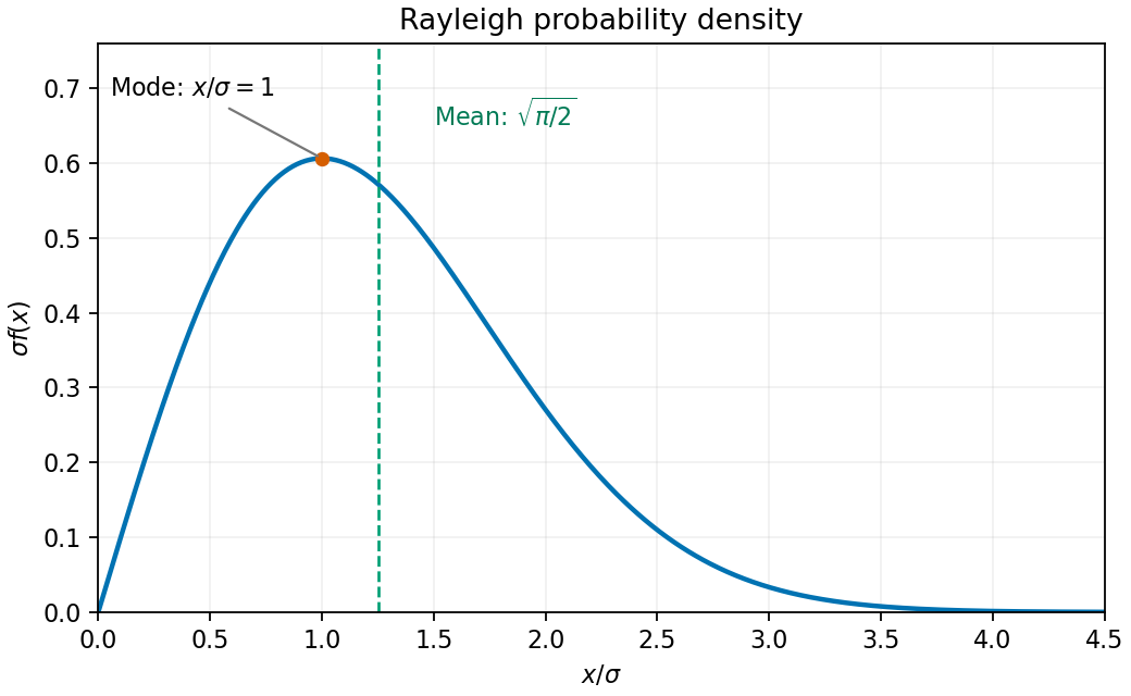
The expected value isIntegrating by parts with $xdx{e}^{-x^2/(2{\sigma }^2)}=-{\sigma }^{2}d(e^{-x^2/(2{\sigma }^2)})$ makes the boundary term vanish and leaves ${\int }_0^{\infty }{e}^{-x^2/(2{\sigma }^2)}dx$. The Gaussian integral gives

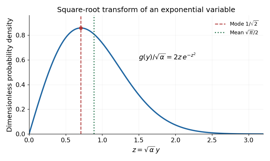
Normalize the probability density function on $x\ge 0$:For $y=\sqrt{x}\ge 0$, the change of variables is $x=y^2$, $dx=2ydy$. Conservation of probability gives the transformed probability density functionIt is a Rayleigh distribution with scale $\sigma =1/\sqrt{2\alpha }$. Its derivative is $g^{\prime }(y)=2\alpha e^{-\alpha y^2}(1-2\alpha y^2)$, so it rises from zero, has one maximum, and then decays:The expected value follows by putting $z=\sqrt{\alpha }y$:Here ${\int }_0^{\infty }{z}^2{e}^{-z^2}dz=\sqrt{\pi }/4$, obtained from the Gaussian integral by integration by parts. In particular $⟨\sqrt{x}⟩\ne \sqrt{⟨x⟩}$, and the mode changes under a nonlinear variable transformation because a density includes its Jacobian determinant.

In an 1880 paper, John William Strutt, known as Lord Rayleigh, studied the resultant of many oscillations with a common frequency and arbitrary oscillation phases. His large-number calculation distinguished a mean intensity from a definite resultant amplitude and used planar coordinates followed by a polar integral. The resulting amplitude density is the Rayleigh distribution in a different scale convention. This is a large-number description, not an exact law for every finite collection of oscillations.^[ref]

To see the connection in a chosen model, take independent oscillation phases ${\Theta }_j$ with uniform distribution on $[0,2\pi )$ and equal component amplitude $a$. The phasor sum has coordinatesBoth have mean zero, variance $n{a}^2/2$ and zero covariance. The multivariate central limit theorem gives an approximately circular Gaussian random vector for large $n$, with $\sigma =a\sqrt{n/2}$. Its amplitude $\sqrt{X_n^2+Y_n^2}$ is therefore approximately Rayleigh. For every finite $n$, that amplitude is bounded by $na$, whereas a Rayleigh distribution has an unbounded tail. At $n=1$ it is exactly $a$. This simple endpoint check prevents the approximation from becoming a false exact identity.

The Rayleigh distribution is the probability distribution of the Euclidean norm of a two-dimensional random vector with independent zero-mean normal random variables of equal variance as components. If $X,Y\sim N(0,{\sigma }^2)$ are independent, thenHere $\sigma$ is the standard deviation of each component, not of the radius $R$. At $\sigma =1$ this gives the unit-scale probability density function $r{e}^{-r^2/2}$.^[ref]

This geometry turns two signed errors into one nonnegative distance. For example, suppose horizontal and vertical positioning errors are independent $N(0,4{\mathrm{cm}}^2)$ random variables. Their means both vanish, but the distance from the intended point is usually positive. The Rayleigh distribution with $\sigma =2\mathrm{cm}$ gives the probability of landing inside any centered disk. These are chosen model assumptions, rather than measurements of a particular instrument.

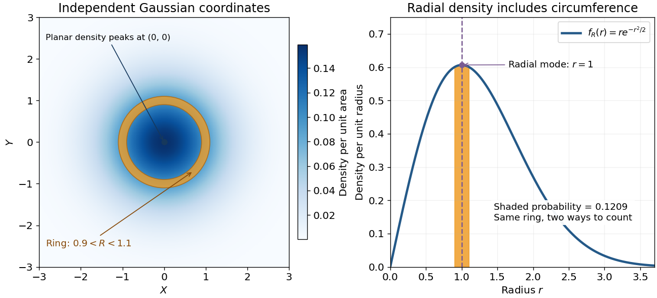
An apparently paradoxical feature is that the most likely location per unit area is the origin, while the radial mode is $\sigma$. A narrow annulus farther out has more area. Near zero that growing circumference outweighs the falling planar density; farther out the exponential function wins. Distinguishing densities measured against different elements of area or length resolves the paradox.

An independent unit-scale Rayleigh distribution variable $R$ and standard normal distribution variable $Z$ give $RZ$ with Laplace distribution of density $e^{-|x|}/2$. Indeed its characteristic function is $\mathbb{E}{e}^{-t^2{R}^2/2}=1/(1+t^2)$.

For $r\ge 0$, integration gives the survival function and cumulative distribution functionSolving $F_R(r_p)=p$ gives the quantile function^[ref]

For the chosen positioning model $\sigma =2\mathrm{cm}$,The disk of radius one component standard deviation therefore contains about 39.35% of outcomes; the familiar one-dimensional normal interval percentage does not apply to a two-dimensional disk. The 95% and 99% radial thresholds areA circle defined by $R=r_p$ itself still has probability zero; its enclosed disk carries the stated probability.

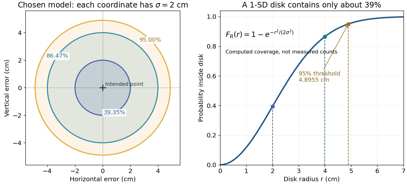
The closed-form quantile function also gives inverse transform sampling: if $U$ has uniform distribution on $(0,1)$, then $\sigma \sqrt{-2\log U}$ has Rayleigh distribution. Using $1-U$ instead gives the same law. Endpoints are excluded so that the logarithm stays finite.

The joint probability density of $X,Y$ isIn polar coordinates, $x=r\cos \theta$, $y=r\sin \theta$, and the absolute Jacobian determinant is $r$. Thus the joint density of radius and angle factors asIntegrating over angle gives the Rayleigh distribution. The same factorization shows that the angle has uniform distribution and is independent of the radius. This is a short change of variables argument: an annulus of width $dr$ has area $2\pi rdr$ to first order.

The assumptions are substantive. Unequal component variances give elliptical rather than circular density contours; a nonzero mean displaces the center. Even zero covariance and equal normal distributions do not suffice without independence. For an original counterexample, let $X\sim N(0,{\sigma }^2)$ and let $S$ be an independent Rademacher random variable. Put $Y=SX$. Then $Y$ has the same normal distribution as $X$, and $\mathrm{Cov}(X,Y)=\mathbb{E}[S{X}^2]=0$. Nevertheless, all points lie on $y=x$ or $y=-x$, and $R=\sqrt{2}|X|$ has densitywhich is positive at zero, unlike the Rayleigh distribution. This pair is not a Gaussian random vector.

Squaring a Rayleigh distribution variable produces an exponential distribution. For $w\ge 0$,where the exponential distribution parameter is a rate. Equivalently, $R^2/{\sigma }^2$ has chi-squared distribution with two degrees of freedom (statistics). An amplitude and its square therefore have different probability density functions, even though one determines the other.

This makes the Rayleigh-normal scale mixture transparent: at unit scale, $R^2$ is exponential, allowing a random normal scale to produce a Laplace distribution. Another equivalent parametrization uses a Weibull distribution with shape two and scale $\sqrt{2}\sigma$. Conventions that call this latter scale the Rayleigh scale differ by a factor of $\sqrt{2}$; check the probability density function before comparing numerical parameter values.^[ref]