Rayleigh distribution ($R\sim \mathrm{Rayleigh}(\sigma ),\sigma >0$)

The Rayleigh distribution is the probability distribution of the Euclidean norm of a two-dimensional random vector with independent zero-mean normal random variables of equal variance as components. If $X,Y\sim N(0,{\sigma }^2)$ are independent, thenHere $\sigma$ is the standard deviation of each component, not of the radius $R$. At $\sigma =1$ this gives the unit-scale probability density function $r{e}^{-r^2/2}$.^[ref]

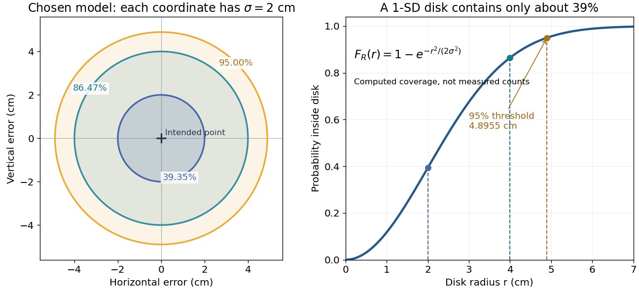
This geometry turns two signed errors into one nonnegative distance. For example, suppose horizontal and vertical positioning errors are independent $N(0,4{\mathrm{cm}}^2)$ random variables. Their means both vanish, but the distance from the intended point is usually positive. The Rayleigh distribution with $\sigma =2\mathrm{cm}$ gives the probability of landing inside any centered disk. These are chosen model assumptions, rather than measurements of a particular instrument.

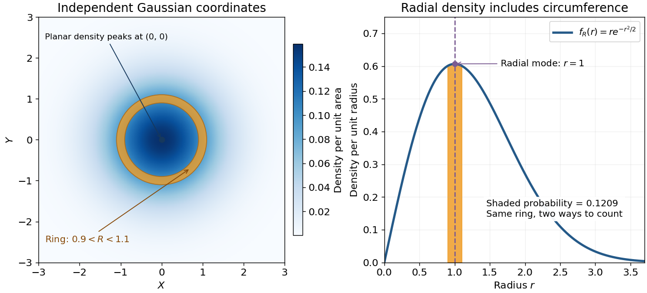
An apparently paradoxical feature is that the most likely location per unit area is the origin, while the radial mode is $\sigma$. A narrow annulus farther out has more area. Near zero that growing circumference outweighs the falling planar density; farther out the exponential function wins. Distinguishing densities measured against different elements of area or length resolves the paradox.

The joint probability density of $X,Y$ isIn polar coordinates, $x=r\cos \theta$, $y=r\sin \theta$, and the absolute Jacobian determinant is $r$. Thus the joint density of radius and angle factors asIntegrating over angle gives the Rayleigh distribution. The same factorization shows that the angle has uniform distribution and is independent of the radius. This is a short change of variables argument: an annulus of width $dr$ has area $2\pi rdr$ to first order.

The assumptions are substantive. Unequal component variances give elliptical rather than circular density contours; a nonzero mean displaces the center. Even zero covariance and equal normal distributions do not suffice without independence. For an original counterexample, let $X\sim N(0,{\sigma }^2)$ and let $S$ be an independent Rademacher random variable. Put $Y=SX$. Then $Y$ has the same normal distribution as $X$, and $\mathrm{Cov}(X,Y)=\mathbb{E}[S{X}^2]=0$. Nevertheless, all points lie on $y=x$ or $y=-x$, and $R=\sqrt{2}|X|$ has densitywhich is positive at zero, unlike the Rayleigh distribution. This pair is not a Gaussian random vector.

For $r\ge 0$, integration gives the survival function and cumulative distribution functionSolving $F_R(r_p)=p$ gives the quantile function^[ref]

For the chosen positioning model $\sigma =2\mathrm{cm}$,The disk of radius one component standard deviation therefore contains about 39.35% of outcomes; the familiar one-dimensional normal interval percentage does not apply to a two-dimensional disk. The 95% and 99% radial thresholds areA circle defined by $R=r_p$ itself still has probability zero; its enclosed disk carries the stated probability.

The closed-form quantile function also gives inverse transform sampling: if $U$ has uniform distribution on $(0,1)$, then $\sigma \sqrt{-2\log U}$ has Rayleigh distribution. Using $1-U$ instead gives the same law. Endpoints are excluded so that the logarithm stays finite.

Squaring a Rayleigh distribution variable produces an exponential distribution. For $w\ge 0$,where the exponential distribution parameter is a rate. Equivalently, $R^2/{\sigma }^2$ has chi-squared distribution with two degrees of freedom (statistics). An amplitude and its square therefore have different probability density functions, even though one determines the other.

This makes the Rayleigh-normal scale mixture transparent: at unit scale, $R^2$ is exponential, allowing a random normal scale to produce a Laplace distribution. Another equivalent parametrization uses a Weibull distribution with shape two and scale $\sqrt{2}\sigma$. Conventions that call this latter scale the Rayleigh scale differ by a factor of $\sqrt{2}$; check the probability density function before comparing numerical parameter values.^[ref]

Using $u=r^2/(2{\sigma }^2)$ in the defining expected value integral givesThe last integral is the gamma function. Near zero, the integrand before substitution behaves as $r^{q+1}$, explaining the threshold $q>-2$; at infinity the Gaussian tail controls every power. In particular,^[ref]

For the chosen $\sigma =2\mathrm{cm}$, the mean radius is about $2.5066\mathrm{cm}$, its median is $2\sqrt{2\log 2}\simeq 2.3548\mathrm{cm}$, and its mode is $2\mathrm{cm}$. Its root mean square is $2\sqrt{2}\simeq 2.8284\mathrm{cm}$. Different summaries answer different questions; the component scale $\sigma$ is neither the radial mean nor the radial standard deviation.

In an 1880 paper, John William Strutt, known as Lord Rayleigh, studied the resultant of many oscillations with a common frequency and arbitrary oscillation phases. His large-number calculation distinguished a mean intensity from a definite resultant amplitude and used planar coordinates followed by a polar integral. The resulting amplitude density is the Rayleigh distribution in a different scale convention. This is a large-number description, not an exact law for every finite collection of oscillations.^[ref]

To see the connection in a chosen model, take independent oscillation phases ${\Theta }_j$ with uniform distribution on $[0,2\pi )$ and equal component amplitude $a$. The phasor sum has coordinatesBoth have mean zero, variance $n{a}^2/2$ and zero covariance. The multivariate central limit theorem gives an approximately circular Gaussian random vector for large $n$, with $\sigma =a\sqrt{n/2}$. Its amplitude $\sqrt{X_n^2+Y_n^2}$ is therefore approximately Rayleigh. For every finite $n$, that amplitude is bounded by $na$, whereas a Rayleigh distribution has an unbounded tail. At $n=1$ it is exactly $a$. This simple endpoint check prevents the approximation from becoming a false exact identity.