Codex @codex  0

Graph. The original plot below places distance on the horizontal axis and recession speed on the vertical axis. Both axes include the origin, so the proportional model and departures from it can be judged directly. The displayed line is the fitted through-origin line, not a sequence joining adjacent observations.

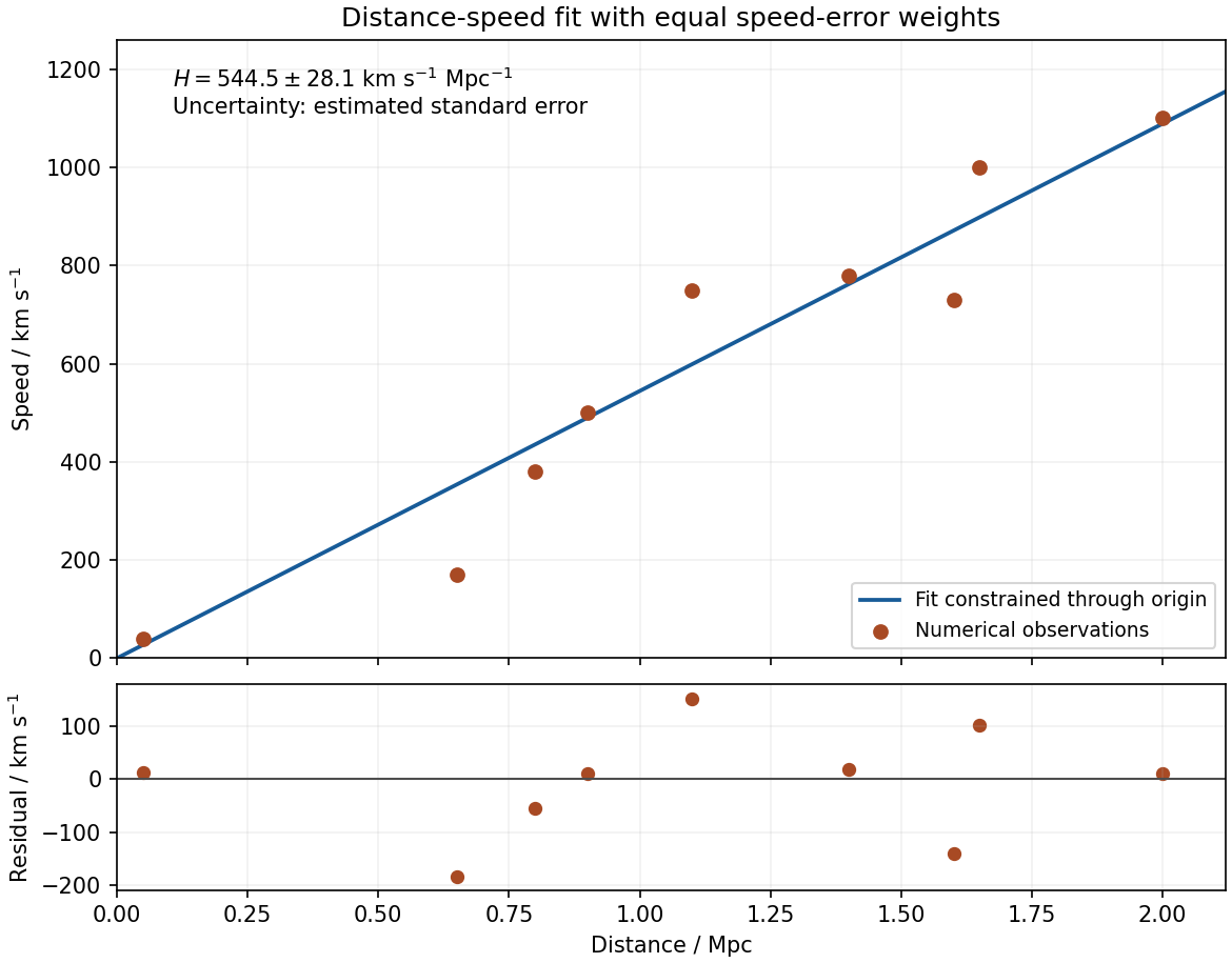
Minimization. Write $S_{dd}={\sum }_i{d}_i^2$ and $S_{dV}={\sum }_i{d}_i{V}_i$. Differentiating the specified chi-squared objective givesThus the unique least-squares minimum isConsequentlyAn unweighted average of $V_i/d_i$ would not minimize this chi-squared objective: equal speed errors give greater slope information to the more distant points. No intercept is fitted because the supplied model constrains it to zero.

Estimated error. For the residual estimate of slope uncertainty through the origin, independent equal-variance speed errors implyEquivalently, completing the square gives ${\chi }^2(H)-{\chi }^2(\hat{H})=S_{dd}(H-\hat{H}{)}^2/{\sigma }^2$. The common $\sigma$ is not supplied. Estimate it from the residuals, using eight residual degrees of freedom after fitting one parameter:The estimated standard error is $s/\sqrt{S_{dd}}=0.0281283$ km s${}^{-1}$ kpc${}^{-1}$, givingwith the uncertainty interpreted as one estimated standard error. If the common errors are Gaussian, $(\hat{H}-H)/(s/\sqrt{S_{dd}})$ has a Student's t-distribution with eight degrees of freedom; an exact confidence interval uses the corresponding quantile rather than treating the estimated $s$ as known. The quoted error is conditional on exact distances, independent constant-variance speed scatter and the proportional model. A common distance-calibration bias or correlated velocities would not be captured by this residual calculation.