Confidence interval ($C(X)=[L(X),U(X)]$)

A confidence interval is a random interval constructed from a statistical sample to cover a fixed unknown statistical parameter with a prescribed coverage probability. For a scalar target $\theta$, a procedure with nominal confidence $1-\alpha$ satisfiesThe subscript records which probability distribution generates the repeated samples. The endpoints are statistics, so they vary from sample to sample; the target is fixed. Equality gives exact nominal coverage probability, while the inequality also permits conservative procedures. For a general estimand $\psi (\theta )$, replace the target inside the interval by $\psi (\theta )$.

A realized confidence interval communicates the precision of an estimate in the target's own units. Reporting $1.2$ alone conceals the difference between an estimate with standard error $0.5$ and one with standard error $0.05$. A narrow confidence interval indicates greater precision for the stated statistical model, rather than a guarantee that its assumptions describe the experiment correctly.

Once $x$ is observed, $C(x)$ either contains the fixed target or does not. The 95% statement concerns the random procedure $C(X)$, not a posterior probability of 0.95 that this particular interval contains $\theta$. A credible interval instead assigns specified posterior probability to a region under Bayesian inference. These interpretations can differ even when the numerical endpoints agree. The repeated-sampling interpretation is explained in NIST's confidence-limits teaching reference.

Jerzy Neyman's 1937 paper formulates the fixed-target, random-endpoint construction in Section II, especially equation (20) on page 348. Its confidence coefficient must hold across the allowed statistical parameters, rather than only at the value suggested by one sample. See Neyman, Outline of a Theory of Statistical Estimation Based on the Classical Theory of Probability and the original paper scan.

Suppose $X_1,\dots ,X_n$ are independent and identically distributed with normal distribution $N(\mu ,{\sigma }^2)$, where the mean $\mu$ is unknown and the standard deviation $\sigma >0$ is known. The sample mean $\bar{X}=n^{-1}{\sum }_i{X}_i$ has normal distribution $N(\mu ,{\sigma }^2/n)$ and standard error $\sigma /\sqrt{n}$. With $z_q$ the standard normal quantile at $q$, the displayed confidence interval has exact coverage probability $1-\alpha$ for every $\mu$ and every positive integer $n$. No central limit theorem approximation is needed.

Take $\sigma =2$, $n=16$ and nominal confidence 95%. The standard error is $2/\sqrt{16}=0.5$, and $z_{0.975}=1.9599639845\dots$. ThereforeRounded for reporting, this is $\bar{x}\pm 0.98$. If $\bar{x}=1.2$, the realized confidence interval is approximately $[0.22,2.18]$. Exact 95% calibration refers to the unrounded standard normal quantile; using $1.96$ literally gives coverage probability $0.9500042097\dots$, almost but not exactly 0.95.

The confidence interval's width scales as $n^{-1/2}$: increasing sample size from 16 to 64 halves its half-width to $0.4899909961\dots$. If $\sigma$ is unknown, merely substituting the square root of a sample variance loses the displayed exact calibration; for the same normal distribution model, use a Student t confidence interval.

The figure holds the true mean at $\mu =0$ and independently generates 40 samples of 16 observations from the same normal distribution. NumPy's PCG64 generator with seed 42 gives 39 covering confidence intervals and one miss, at sample 32: observed coverage is $39/40=97.5\%$. Every bar uses the unrounded standard normal quantile. This finite collection illustrates the moving endpoints; it does not establish the analytic coverage probability or require exactly two misses.

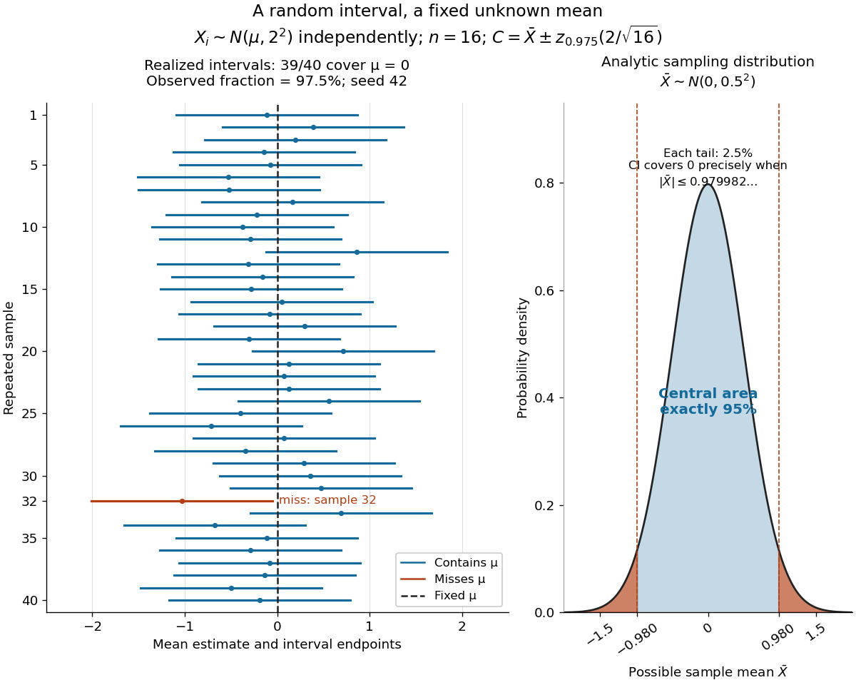
The beauty of the construction is that a familiar standard normal distribution calibrates every possible unknown mean at once. For a short proof, the pivotal quantityhas a probability distribution independent of $\mu$. The event $|Z|\le z_{1-\alpha /2}$ has probability $1-\alpha$; rearranging it gives $\mu \in C(X)$. The right panel shows the equivalent event $|\bar{X}|\le 0.9799819923\dots$ when $\mu =0$.

For the same normal distribution model, a two-sided test compares the null hypothesis $H_0:\mu ={\mu }_0$ with the alternative hypothesis $H_1:\mu \ne {\mu }_0$. Under the null hypothesis, the standardized test statistic has standard normal distribution. Write $\Phi$ for the standard normal distribution function. With $\bar{x}=1.2$, $\sigma =2$, $n=16$ and ${\mu }_0=0$, the observed test statistic is $z=1.2/0.5=2.4$. Its p-value isThus the p-value is a tail probability computed under the null hypothesis, including departures in both directions. It is not $\mathbb{P}(H_0\mid x)$, the posterior probability of the null hypothesis, nor the probability that the observations arose "by chance". The normal distribution test statistic and its calibration appear in NIST's teaching reference for testing a process mean; the tail interpretation is stated in Penn State's hypothesis-testing notes.

Choose the significance level $\alpha =0.05$ before observing the sample. The rejection region is $|Z|>z_{0.975}$, whose probability under $H_0$ is exactly 0.05. Here $2.4>1.9599639845\dots$, so reject $H_0$. This agrees with zero lying outside $[0.22,2.18]$. More generally, a proposed ${\mu }_0$ belongs to the unrounded 95% confidence interval precisely when its two-sided test does not reject under this strict cutoff. The equality boundary has probability zero in this continuous statistical model.

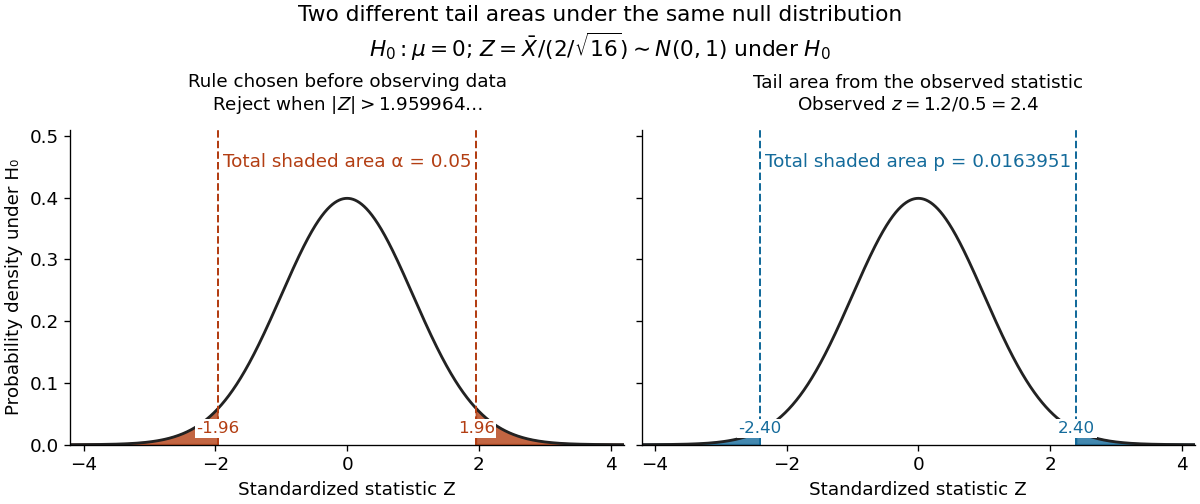
The significance level and statistical power describe different repeated-experiment probabilities. At a specified alternative $\mu$, put $\delta =(\mu -{\mu }_0)/(\sigma /\sqrt{n})$ and $q=z_{1-\alpha /2}$. ThenThe first is the Type I error probability; the second is the Type II error probability at that alternative. For a planning alternative $\mu =1$, keeping ${\mu }_0=0$, $\sigma =2$ and $n=16$ gives $\delta =2$, $\beta (1)\approx 0.483995$ and statistical power $0.516005$. At $n=64$, $\delta =4$ and statistical power rises to $0.979327$. These are model calculations for specified alternatives, not posterior probabilities inferred from a nonsignificant result. They explain why failure to reject cannot establish equality and why choosing sample size before an experiment is useful.

Historically, Ronald Fisher's 1925 book discusses the normal cutoff $1.96$ and tail probability 0.05 as a convenient convention on page 47, rather than a mathematically compulsory threshold: ^[ref].

The coverage probability is the repeated-sampling probability that a random confidence interval contains the fixed true statistical parameter. A finite-sample level-$1-\alpha$ procedure has coverage probability at least $1-\alpha$ at every admissible statistical parameter; exact nominal coverage means equality. An asymptotically calibrated procedure approaches the nominal value as sample size grows, under its stated assumptions. Higher-order Edgeworth expansions can quantify the discrepancy from nominal coverage probability when their regularity conditions hold.

Observed coverage in finitely many repetitions is itself random. For $m$ independent repetitions of the exact normal mean confidence interval with known variance, the count $K$ of covering confidence intervals has binomial distribution $\mathrm{Binomial}(m,0.95)$. At $m=40$, its expectation is $38$, butConsequently, the 39 successes in the figure are compatible with exact 95% coverage probability. The guarantee follows from the pivotal quantity's probability distribution; the finite observed fraction is an illustration. Also distinguish a confidence interval for a fixed mean from a prediction interval for a future observation: the latter must accommodate the new observation's variation as well as estimation uncertainty.

The sample minimum and maximum enclose random population content given by the uniformized sample range. The exact failure probability for content at least $1-\epsilon$ is $(1-\epsilon {)}^{n-1}[1+(n-1)\epsilon ]$. For small $\epsilon$, setting $n\epsilon \approx \vartheta$ gives the displayed sample-size approximation at confidence $1-\delta$. The positive solution is unique for $0<\delta <1$, since $(1+\vartheta )e^{-\vartheta }$ decreases from one to zero. A tolerance interval concerns population content, rather than a confidence interval for a fixed parameter; the exact inequality should select the final integer size.

For an exponential distribution with mean $\theta$, the maximum-likelihood estimator is $\bar{Y}$ and $\sqrt{n}(\bar{Y}-\theta )/\theta$ converges to a standard normal distribution. Inverting the event that this pivot lies between $-z$ and $z$ gives the displayed confidence interval, provided $n>z^2$. Its two-sided coverage probability has error $O(n^{-1})$, because the first Edgeworth expansion term is even and cancels between the two tails.

For jointly approximately normal estimates $(\hat{C},\hat{E})$ with estimated variances $v_C,v_E$ and covariance $v_{CE}$, a confidence interval for the ratio $C/E$, where $E\ne 0$, can be obtained by inverting tests of $C-rE=0$. For each proposed ratio $r$, the contrast has estimate $\hat{C}-r\hat{E}$ and variance $v_C-2r{v}_{CE}+r^2{v}_E$. Retain $r$ when its absolute standardized contrast is at most the chosen critical value $q$. This gives the displayed quadratic inequality, with coefficients $A={\hat{E}}^2-q^2{v}_E$, $B=-2(\hat{C}\hat{E}-q^2{v}_{CE})$, $D={\hat{C}}^2-q^2{v}_C$. When $A>0$ and the discriminant is positive, retain the interval between the roots. When $A<0$, a confidence set can instead be two unbounded rays or the entire real line. Degenerate linear cases are interpreted directly from the inequality. A bounded interval must not be forced when the denominator is poorly separated from zero. Known covariance matrix and a joint normal distribution give exact normal critical values; estimated covariance usually gives approximate coverage, unless an appropriate exact common-scale pivot exists.

A lower confidence bound $L$ gives a one-sided confidence interval with the displayed coverage requirement for every admissible parameter. An upper bound $U$ instead satisfies ${\mathrm{Pr}}_{\theta }\{\theta \le U\}\ge 1-\alpha$. Coverage is a repeated-sampling property; it does not assign a posterior probability to the fixed parameter.

Invert a likelihood-ratio test for a scalar parameter, maximizing over nuisance parameters for each fixed candidate value. Under regularity, a level $1-\alpha$ interval includes values whose profile log-likelihood is at most ${\chi }_{1,1-\alpha }^2/2$ below its maximum. This explains the horizontal cutoff on a Box–Cox transformation likelihood plot.

If a positive rate $q$ has a confidence interval $[L,U]$, monotonicity transforms it into $[1/U,1/L]$ for the reciprocal mean $1/q$. This preserves the coverage event exactly and reverses the endpoints. It applies directly to mean exponential holding times.

For a sample of size $n$ from a continuous probability distribution, this interval covers the median $F^{-1}(1/2)$ with probability $1-2{\sum }_{r=0}^{j-1}\left(\genfrac{}{}{0ex}{}{n}{r}\right)2^{-n}$, for $1\le j<n/2$. Count observations below the median: their number has the binomial distribution with parameters $n,1/2$. No strict increase of the distribution function is needed.

For two independent observations uniform on $[\theta -a,\theta +a]$, the displayed interval of possible parameter values contains the true parameter almost surely. Intersecting any confidence interval with it preserves that interval's coverage, while excluding values inconsistent with the observations. The order statistics interval $[U_{(1)},U_{(2)}]$ has coverage $1/2$, since the observations straddle $\theta$ with probability $1/2$. If their separation exceeds $a$, the entire interval of possible parameters lies between the observations; this explains why the nominal one-half procedure can be unnecessarily wide on that event.