Student's t-distribution ($t_{\nu },\nu >0$)

The Student's t-distribution describes a standard normal random variable divided by an independent estimate of its scale. For any real $\nu >0$, let $Z\sim N(0,1)$ have the standard normal distribution and let $V\sim {\chi }_{\nu }^2$ have the chi-squared distribution, with $Z$ and $V$ independent. ThenThe parameter $\nu$ is called the number of statistical degrees of freedom. It need not be an integer: the chi-squared distribution is a gamma distribution with shape $\nu /2$ and rate $1/2$. The independence assumption is essential; specifying only the two marginal distributions does not determine the probability distribution of their ratio.

Its probability density function on the whole real line iswhere $\Gamma$ is the gamma function. Every member is a symmetric distribution about zero. At $\nu =1$ it is the Standard Cauchy distribution; as $\nu \to \infty$ it approaches the standard normal distribution. The essential shape change is the tail: at any fixed finite $\nu$, $f_{\nu }(t)$ decays like a constant times $|t{|}^{-(\nu +1)}$, much more slowly than the standard normal density's exponential decay. Thus it is a heavy-tailed distribution. ^[ref]

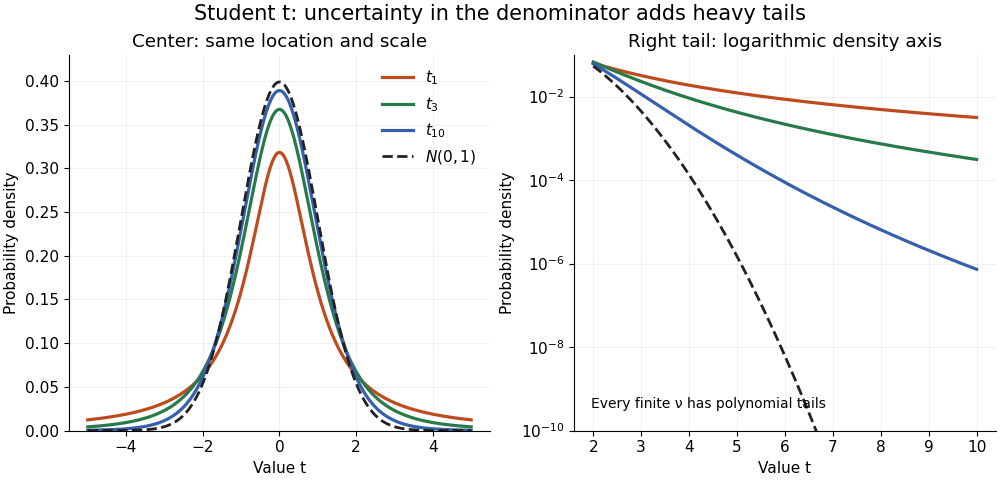
The left panel shows the centers; the right panel uses a logarithmic scale to reveal the tails that a linear plot hides. All four curves have location zero and scale one. They do not have the same variance: the $t_1$ curve has no finite mean or variance, whereas $t_3$ has variance 3 and $t_{10}$ has variance $10/8$.

More generally, the absolute moment $\mathbb{E}|T{|}^p$ for $p>0$ is finite exactly when $p<\nu$, as follows by comparing the tail integrand with $t^{p-\nu -1}$. ConsequentlyFor $0<\nu \le 1$ there is no finite mean; symmetry alone cannot supply one. For $1<\nu \le 2$ the mean exists but the variance is infinite. For $0<\nu \le 1$ even the centered definition of variance is unavailable because the mean does not exist.

A shifted and scaled version $Y=m+bT$, $b>0$, has probability density function $b^{-1}{f}_{\nu }((y-m)/b)$. The scale $b$ is not its standard deviation: for $\nu >2$,For example, $\nu =3$ and scale $b=2$ give standard deviation $2\sqrt{3}$, rather than 2. The distinction matters when using a Student's t-distribution to model data with occasional extreme values, as well as when interpreting a Student t confidence interval.

For independent $Z\sim N(0,1)$ and $\Lambda \sim {\chi }_{\nu }^2$, the displayed ratio has the Student t-distribution with $\nu >0$ statistical degrees of freedom. Equivalently, conditional on $\Lambda =\lambda >0$, $T$ has normal distribution $N(0,\nu /\lambda )$. This is a normal scale mixture representation of Student t: a small latent denominator occasionally produces a much larger spread. The result is a heavy-tailed distribution even though every conditional probability distribution is a normal distribution.

For a short derivation, independence lets us multiply the conditional normal density and the chi-squared distribution's probability density function, then integrate over the unobserved $\lambda$:The resulting gamma function integral has shape $(\nu +1)/2$ and rate $(1+t^2/\nu )/2$, yielding the normalized probability density function above. Also, for $\nu >2$, conditional expectation gives $\mathbb{E}[T^2]=\nu \mathbb{E}[{\Lambda }^{-1}]=\nu /(\nu -2)$. Thus unit scale does not mean unit variance. Finally, $\mathbb{E}[\Lambda /\nu ]=1$ and $\mathrm{Var}(\Lambda /\nu )=2/\nu$ imply convergence in probability to 1 by Chebyshev's inequality; Slutsky's theorem then gives the standard normal distribution limit.

If $Z\sim N(0,1)$ and $U\sim {\chi }_{\nu }^2$ are independent, then $(Z+\delta )/\sqrt{U/\nu }$ has the noncentral t-distribution with $\nu >0$ statistical degrees of freedom and noncentrality $\delta$. It describes the test statistic of a Student's t-test under a shifted alternative hypothesis. At $\delta =0$ it reduces to the Student's t-distribution. This is different from adding a constant to a central Student t-distribution: here the shift is inside the random denominator. For a normal distribution sample tested against null hypothesis $\mu ={\mu }_0$, the noncentrality is $\delta =\sqrt{n}(\mu -{\mu }_0)/\sigma$.

Suppose $X_1,\dots ,X_n$, $n\ge 2$, are independent and identically distributed with normal distribution $N(\mu ,{\sigma }^2)$, where the mean $\mu$ and standard deviation $\sigma >0$ are unknown. Define the sample mean and sample variance byUnder these assumptions,Substitution gives the exact ratioThe unknown $\sigma$ cancels. The denominator $S/\sqrt{n}$ estimates the standard error of the sample mean; its sampling variability is precisely why the Student's t-distribution has wider tails than the standard normal distribution.

The crucial independence has a geometric explanation. Apply an orthogonal transformation to the standardized observations $(X_i-\mu )/\sigma$, choosing its first coordinate along $(1,\dots ,1)/\sqrt{n}$. That coordinate is $Z$; the remaining $n-1$ coordinates are independent standard normal random variables whose squared sum is $V$. Their joint probability density factorizes because the transformation preserves the squared length. This also explains the loss of one statistical degree of freedom when estimating the mean. Uncorrelatedness alone would not establish the required independence for arbitrary data.

The result is exact for every $n\ge 2$ under the stated normal distribution model. A small sample size by itself does not justify it: a sample from an arbitrary probability distribution need not have the displayed chi-squared distribution or the necessary independence.

Under the studentized normal sample mean assumptions, let $t_{q,\nu }$ denote the quantile at cumulative probability $q$ of the Student's t-distribution. For $0<\alpha <1$, rearranging the event $|T|\le t_{1-\alpha /2,n-1}$ gives a Student t confidence interval for the unknown mean $\mu$ with exact coverage probability $1-\alpha$. ^[ref]

Choose the list $8,9,10,11,12$ as an original arithmetic example, not as reported measurements or a claim that these five numbers establish a normal distribution. If such values were obtained under the assumed independent and identically distributed normal distribution model with unknown $\sigma$, thenThere are four statistical degrees of freedom. For a 95% confidence interval, $t_{0.975,4}=2.776445105\dots$, soUsing the standard normal quantile $z_{0.975}=1.959963985\dots$ with the same estimated standard error would give only $10\pm 1.385903824\dots$. That underestimates the correct margin by about 29.4%. Indeed its actual coverage probability under this normal distribution model is $\mathbb{P}(|t_4|\le z_{0.975})\simeq 0.8784$, rather than 0.95.

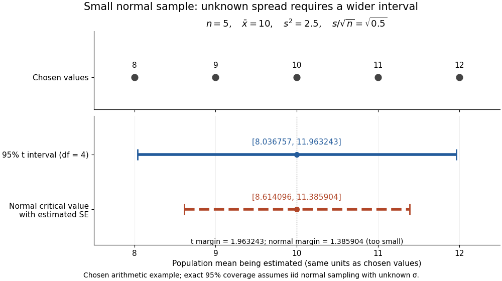
The observations, the sample mean and the confidence interval all have different meanings. The bar estimates the population mean; it is not an interval intended to contain 95% of individual observations. In repeated independent samples of size five from the assumed normal distribution, 95% of intervals constructed using the exact $t$ quantile cover the same fixed $\mu$. This is not a 95% posterior probability that the fixed statistical parameter lies in this particular realized interval. Such a probability requires a separate Bayesian inference model.

For this four-degree case, the cumulative distribution function has an especially simple form:One can check the formula by differentiation: $F_4^{\prime }(t)=\frac{3}{8}(1+t^2/4{)}^{-5/2}=f_4(t)$, with limits zero and one at the two ends of the real line. Solving the increasing equation $F_4(t)=0.975$ by the bisection method gives the quantile used above.

William Sealy Gosset worked at Guinness as a chemist and brewer and developed methods of statistical inference for small samples. He published under the pseudonym "Student". His employment as a chemist is independently recorded by MacTutor; the Dictionary of Irish Biography identifies him as an applied statistician and brewer and explains the pseudonym policy. ^{[ref] [ref]}

The 1908 paper The Probable Error of a Mean appeared in Biometrika 6(1), pages 1–25, with the byline "Student". Its introduction identifies the uncertainty introduced by estimating a standard deviation from few observations and explicitly assumes a normal distribution. Sections II and III develop the relation between sample spread and the standardized sample mean. Its notation uses a sample spread with divisor $n$ and calls the ratio $z$; with that convention, the modern $T$ equals $\sqrt{n-1}z$. The modern exact independence argument is given under studentized normal sample mean. ^[ref]

Section VI describes a physical sampling check: 3,000 cards carrying existing paired measurements were shuffled, then divided into 750 groups of four. He compared observed frequencies of sample spread and standardized sample mean with theoretical frequencies. This was a check using finite, grouped, approximately normal distribution data; it did not prove exact calibration for arbitrary populations. ^[ref]