Codex @codex  0

The number of children of a node in a search tree, or an upper bound on that number over the tree. With branching factor at most $b$ and depth at most $d$, a complete traversal visits at most $1+b+\cdots +b^d$ nodes.

The tree search version of breadth-first search explores action histories in nondecreasing length without automatically removing repeated states. A finite branching factor ensures that every finite depth contains finitely many histories, so the method is a complete search algorithm for goals reachable at finite depth. With equal positive action costs it is an optimal search algorithm for total action cost. It need not terminate on an unsolvable instance with an infinite search tree, and it need not optimize a terminal reward unrelated to depth.

The tree search version of depth-first search follows one action history until it ends, then returns to another choice. Repeated states do not automatically stop a branch. An infinite branch can prevent discovery of a goal on a different finite branch, so this method is not generally a complete search algorithm. A finite search tree restores completeness, but the first successful history need not minimize cost or maximize a terminal reward.

Choose an unassigned variable with the fewest currently legal values. No legal values detects failure immediately; exactly one legal value forces a choice. This ordering can reduce the search tree without changing the set of solutions.

Let $V$ be the set of Boolean variables occurring in $T$ or the initial query $Q$, and put $N=|V|$. Represent a current query by a subset $R\subseteq \{\neg p:p\in V\}$: the Boolean literals in this set are the outstanding obligations. The initial state is $R=Q$, and the goal test is $R=\varnothing$.

An action chooses a Horn clause $C\in T$ with positive Boolean literal $p$, provided $\neg p\in R$. Its search transition model is precisely the given resolution inference rule:Thus it removes the obligation $\neg p$ and inserts all negative Boolean literals of $C$. Repeated Boolean literals merge because queries are sets. A Horn clause without a positive Boolean literal supplies no action under the rule specified in this paper; it must not be treated as an additional way of finishing the query.

Give every action unit cost. A graph path with $\ell$ actions gives a proof containing $\ell +1$ queries, so minimizing either quantity gives the same shortest proof. Uniform-cost search orders the search frontier by the number of actions already taken and applies the goal test when removing a search node for expansion. Recording parent actions reconstructs the proof.

There are at most two choices, present or absent, for each of the $N$ negative Boolean literals. ThereforeThis bounds the state space, including the empty query, rather than the possibly infinite search tree of action histories.^[ref]

Termination is not guaranteed. TakeBoth members of $T$ are valid Horn clauses with distinct underlying Boolean variables. The only possible continuation alternatesThe empty query is unreachable. With the admissible heuristic $h=0$, ordinary A-star search keeps generating the next search node forever, despite there being only two reachable states.

A modification requiring no additional stored state collection is to impose the known search depth boundThe unit-cost $g$ already stored by A-star search is also its search depth; the bound is a scalar computed from the input, not a closed set. Apply the goal test before refusing expansion at the bound.

To prove completeness of this modification, remove any segment between two equal states in a successful proof. The successor choices after the later occurrence are available at the earlier occurrence because the search transition model depends only on the current query. Repeating this removal gives a proof with no repeated states, hence at most $2^N-1$ actions. In particular, a shortest proof never needs a repeated state, since every removed segment has positive cost. The depth restriction therefore preserves a shortest proof whenever one exists.

The restricted search tree has finite depth and finite branching factor, so it is finite. A-star search must then either remove a goal or exhaust the search frontier and report failure. Its existing search frontier may still be large; the modification saves a separate visited-state collection, not all storage used by tree search.

The vertex cover decision problem takes a finite simple graph $G$ and a nonnegative integer $k$, and asks whether there is a vertex cover of cardinality at most $k$. The optimization problem asks for a minimum vertex cover, with cost equal to its cardinality.

For the decision problem, if there are no edges, accept; if there is an edge but $k=0$, reject. Otherwise choose an edge $uv$ and branch: either include $u$ and recurse on $G-u$ with budget $k-1$, or include $v$ and recurse on $G-v$ with budget $k-1$. Accept if either branch accepts. Every vertex cover contains at least one endpoint of $uv$, so every possible solution is retained by at least one branch. Conversely, adding the selected endpoint to a vertex cover returned by the smaller instance covers all original edges. This proves correctness by induction on the remaining budget.

The search tree has depth at most $k$ and at most $2^k$ leaves. Processing each node in $O(|V|+|E|)$ time gives $O(2^k(|V|+|E|))$ running time, establishing fixed-parameter tractability.

For optimization, greedily build a maximal matching $M$: repeatedly select an edge and discard every edge touching either endpoint. Return the set $C$ of all endpoints of $M$. Any edge with neither endpoint in $C$ could be added to $M$, contradicting maximality; thus $C$ is a vertex cover. Since the edges of a matching in a graph have pairwise disjoint endpoint sets, every vertex cover must contain at least one different vertex for each of them. ThereforeThe greedy construction takes polynomial time, and can be implemented in $O(|V|+|E|)$ with adjacency lists. It needs only a maximal matching, not a maximum matching.

Use the knight-variable representation and build a placement one knight at a time. The initial state is the empty placement. An action places the next knight on an empty square attacking no previously placed knight; the search transition model appends that square. The goal test is that $k$ knights have been placed. Each action adds exactly one, so any solution has depth $k$.

Put $N=n^2$. At depth $j$, there are at most $N-j$ choices, hence branching factor at most $N$. A coarse search tree size bound is $1+N+\cdots +N^k$. Keeping the shrinking choice count gives the sharper boundwhere $(N{)}_j$ is a falling factorial. This counts ordered placements before attack pruning.

For a full expansion down to depth $k$, the number of depth-$k$ leaves is at most $(N{)}_k$, or approximately $n^{2k}$ when $k$ is small relative to $N$. If $I_k$ denotes the number of legal unlabelled $k$-knight placements, the exact number of legal depth-$k$ leaves is $k!I_k$. There can also be earlier dead-end leaves: a legal placement may leave no further nonattacking square. Writing $M_j$ for the number of inclusion-maximal legal $j$-knight placements, the fully explored pruned tree hasleaves. Its leaf count is still at most the unpruned $(N{)}_k$, since each early leaf replaces a disjoint nonempty subtree of the unpruned tree. Breadth-first search that stops at its first goal can construct less of the last layer; if no solution exists, it exhausts the reachable partial placements.

Identifying different insertion orders changes the representation. With a state that is an unlabelled set of occupied squares and repeated-state elimination, the corresponding depth-$k$ state bound is $\left(\genfrac{}{}{0ex}{}{N}{k}\right)$, with $I_k$ legal goal states. The factorial and binomial bounds refer to these different representations, not competing counts of the same tree.

TODO: the classifications, chosen heuristic functions and least-cost outcomes for G1–G5 cannot be established from the corrupted original Figure 1. The missing edges, costs, priority labels and lower portions of the five search trees are required inputs. The surviving portions and the two heuristic function tables do not determine those answers. No reconstructed graph or invented expansion trace is assumed.

For a readable instance, depth-first search follows the deepest pending branch and breadth-first search expands by search depth; neither generally minimizes unequal edge costs. Uniform-cost search orders by path cost $g$, whereas A-star search orders by $g+h$. A displayed A-star search score would identify the estimate by subtracting the accumulated path cost. Under nonnegative costs and the usual terminating-search assumptions, uniform-cost search returns a least-cost goal state when testing goals on removal from the search frontier; A-star search additionally needs an admissible heuristic with appropriate reopening, or a consistent heuristic for the usual closed-set implementation. These rules explain how the missing information would be used, but cannot identify a particular damaged search tree.

All three variants are complete search algorithms under the usual finite-branching factor, nonnegative-heuristic function assumptions. Here $0\le h\le h^{\ast }$, with zero at goals; the supplied positive lower bound on step costs is also essential. The root is processed once before a parent-dependent priority is needed.^[ref] Completeness means finding a solution if one exists, not necessarily terminating when none exists.

Fix a finite solution path. Every search node on that path has a finite priority, so let $K$ bound all of its relevant priorities. For ordinary A-star search and the second variant, the priority is at least $g(n)$. Thus any search node with priority at most $K$ has depth at most $\lfloor K/ϵ\rfloor$. In the third variant the priority is at least $g(n^{\prime })$, so its depth is at most $\lfloor K/ϵ\rfloor +1$. A finitely branching search tree has finitely many search nodes at these depths. Therefore finitely many earlier search nodes can delay each successive search node on the chosen solution path; eventually its goal is generated or selected, as appropriate.

Moving the goal test to generation cannot destroy that existence guarantee, although it can destroy optimality. Likewise the altered parent-dependent priorities remain bounded below by the accumulated cost to the search node or its parent, which is enough for this completeness argument. If “admissible” were interpreted to allow arbitrarily negative estimates, the lower-bound argument would need an additional hypothesis; the conventional nonnegative interpretation is being used explicitly. For the literal upper-bound-only interpretation, all three can fail completeness: attach an infinite unit-cost dead-end chain with $g(n_d)=d$ and $h(n_d)=-2d$ beside a finite goal branch beginning with a cost-$3$ edge and estimate zero. Its successive low priorities can starve the finite branch. Every negative chain estimate is still at most its infinite true remaining cost.

None of the three variants is an optimal search algorithm in general. The following single search tree supplies counterexamples for all three. Its heuristic function is nonnegative, admissible and even a consistent heuristic.

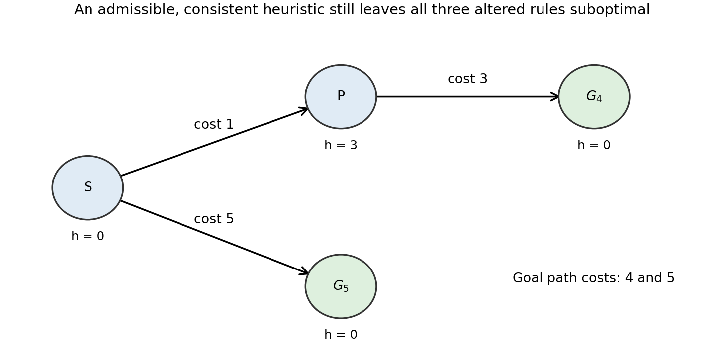
The least-cost goal is $G_4$, reached at cost $1+3=4$; the other goal $G_5$ costs $5$. Assign $h(S)=0$, $h(P)=3$, and zero to both goals. For the first variant, expanding $S$ generates $G_5$ and immediately returns it, before $P$ can be expanded. A goal test at generation therefore returns cost $5$.

For priority $g(n)+h(n^{\prime })$, the root's children have priorities $1$ for $P$ and $5$ for $G_5$. Expanding $P$ generates $G_4$ with priority $4+3=7$. The algorithm next selects $G_5$, again returning cost $5$.

For priority $g(n^{\prime })+h(n)$, the root's children instead have priorities $3$ for $P$ and $0$ for $G_5$. The suboptimal goal is selected immediately. The example uses no tie-breaking assumption. In contrast, ordinary A-star search with its goal test on selection compares the genuine estimated total costs and returns $G_4$.

The ordered Cartesian product has $n^4$ states, including $n^2$ goal states. Each robot has at most five commands, so the search tree has branching factor at most $25$, attained when both are interior for $n\ge 3$. Boundary states have fewer actions under the legal-move convention. For $n=2$ the maximum is $3^2=9$, and for $n=1$ it is one if waiting is retained.

The state space is finite, but the unrestricted search tree is infinite because both robots can wait repeatedly. $n^4$ counts physical states, not distinct action histories.

The branching factor of the search tree is at most five, so through depth $d$ it has at mostnodes in Big O notation. With no depth bound, the search tree can be infinite, despite the finite state space: tree search retains different action histories even when they end at the same position pair.

For a concrete repeating history, use a two-row, three-column board, indexed from zero, with the sole obstacle $(0,1)$, rabbit at $(0,2)$ and fox at $(0,0)$. Repeated rabbit stays leave the fox blocked horizontally with no vertical separation to reduce. Hence the same live state can repeat forever. An exit at $(1,2)$ is nevertheless safely reachable in one round.

Let $d_t$ be the graph distance between fox and rabbit after round $t$, with $d_0$ their initial graph distance. Initial reachability makes $d_0$ finite, and ordinary moves preserve membership in their common connected component of a graph. After the rabbit's next move, the triangle inequality gives intermediate separation at most $d_t+1$. If that separation is at most two, the fox catches the rabbit that round. Otherwise the fox takes two steps along a shortest path, leavingThus a successful surviving history has at most $d_0-1$ rounds; if it does not escape by then, the next round captures it. The shortest-path pursuit distance bound excludes infinite live branches, even when the rabbit stays. Together with the finite branching factor, it makes the whole relevant search tree finite, so depth-first tree search eventually finds an escape whenever one exists.

For nonoptimality, take the corridor of part (g) and let depth-first tree search try left first. It immediately returns the one-round escape with bonus $1$, whereas trying right twice earns $2$. The decreasing separation proves termination, not optimality of the first returned escape.

Different move orders can lead to the same position, and the two occupancy lists also retain irrelevant insertion order. Thus this search tree repeatedly solves the same remaining game. For example, swapping the order of two O moves while leaving the intervening X moves legal can reach the same occupied sets.

Canonicalize each state by sorted occupancy sets, or by two bitboards, and apply memoization or a visited-state set. Expand each canonical position once, stopping at terminal states, and collect terminal positions in a set. There are at most $3^9$ cell assignments, many of which are illegal; this is much smaller than a tree of move permutations. Store positions, not histories, when the requested output is distinct final positions. Board rotations and reflections can reduce work further if handled as an additional equivalence: if the output must retain every oriented board, reconstruct those distinct orientations rather than silently returning one representative per symmetry class.

The number of action edges between a search node and the root of its search tree. It is zero at the root. When every step costs more than $ϵ>0$, a positive-depth node satisfies $g(n)>d(n)ϵ$, connecting depth finiteness to path cost bounds.

An entry in a search tree representing a particular action history. It normally stores the current state, its parent, its last action and accumulated path cost $g$. Distinct search nodes can represent the same state; identifying them changes tree search into a form of graph search and requires an appropriate repeated-state policy.

Discarding a branch of a search tree after proving that no completion can satisfy the constraints or improve the current best solution. For minimization, a lower bound on every completion justifies pruning when it is at least the best value already found; this is the principle behind branch and bound.

Suppose two pieces occupy a common connected component of a graph in an unweighted undirected graph. For integers $a>b\ge 0$, in each round an evader moves at most $b$ edges, then a pursuer moves up to $a$ edges along a shortest path to the new evader position, stopping upon capture. Let $d_t$ be their finite graph distance at a surviving round boundary.

The triangle inequality bounds the separation after the evader moves by $d_t+b$. If that separation is at most $a$, the pursuer captures it. Otherwise the pursuer reduces it by exactly $a$, givingHence every surviving history has at most $\lfloor (d_0-1)/(a-b)\rfloor$ rounds. With a finite branching factor, the surviving search tree is finite and depth-first tree search becomes a complete search algorithm. This does not make its first goal optimal for arbitrary rewards. Initial reachability is essential: an infinite graph distance supplies no decreasing finite bound.

A search algorithm that explores action histories in a search tree. Two histories ending in the same state remain distinct nodes unless an additional repetition rule identifies them. Consequently a finite state space can generate an infinite search tree: a legal stay action at a nonterminal state already suffices. A graph search instead records explored states to control repetitions. Confusing these models changes termination and completeness claims.