An adjacency list represents a graph by keeping, for each vertex , a collection of the vertices reached by its outgoing edges. An array indexed by vertex identifiers can locate each collection; the collection itself may use a linked list or an array. In an undirected graph, each nonloop edge supplies an entry at both endpoints.[ref]
Graph.java. Graph.java, class documentation and fields: vertex-indexed adjacency collections; addEdge: entries at both endpoints
For a worked example, take the simple graphwhere denotes the unordered pair . Its adjacency lists, displayed in label order, areThus has three neighbours, although the graph has six vertices. Its list contains exactly the destinations available for a single step from ; no slots are reserved there for . The fourteen neighbour entries represent seven edges, with appearing as in 's list and as in 's list. The label order makes the example easy to read; an adjacency list need not be sorted.
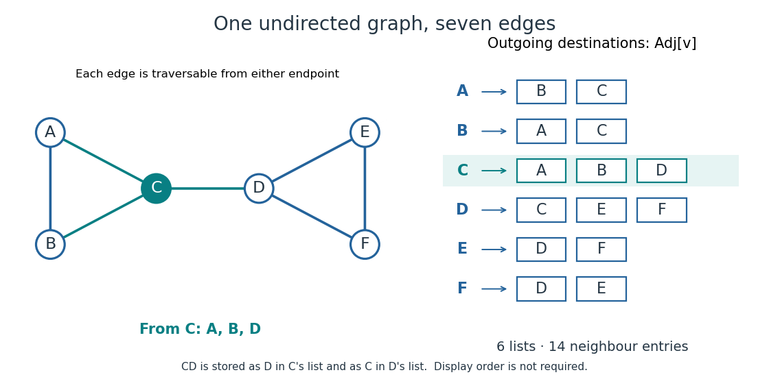
Seven undirected edges and their fourteen adjacency list entries
. Details. The useful idea is to store existing connections explicitly. Neighbour enumeration can then follow exactly the possible next steps, which is what breadth-first search and depth-first search need. In a sparse graph, most pairs of vertices have no edge; adjacency lists avoid reserving a separate adjacency matrix entry for every such absence. Whether this saves work depends on the question: neighbour enumeration and testing one proposed edge have different costs.
For a directed graph, store in for the edge . The reverse edge is separate and is stored only if it exists. Consequently, list length is outdegree, not indegree, and each directed edge contributes one entry in total. An incoming-list index is additional storage.[ref]
Digraph.java. Digraph.java, addEdge, adj and outdegree: one entry in the tail's collection; indegree is maintained separately
Orient the seven edges of our example from earlier to later labels. The resulting directed graph hasThere are now seven entries, with outdegrees . In particular, needs an empty list even though it is reached from : incoming edges do not make 's outgoing list nonempty. Replacing each directed edge by an undirected graph connection would lose this distinction.
Our running simple graph excludes self-loops and repeated edges. If those restrictions are relaxed, specify how the adjacency list encodes them. Here an undirected self-loop at contributes two copies of to , matching its contribution of two to the degree of a vertex. A directed self-loop contributes one copy, and one each to outdegree and indegree. Distinct parallel edges retain distinct entries; a multigraph's list length can therefore exceed its number of distinct neighbours.[ref]
Graph.java. Graph.java, class documentation: parallel edges and two-entry undirected self-loop convention; addEdge applies both insertions even when v equals w
[ref]Digraph.java. Digraph.java, class documentation and addEdge: parallel edges permitted; a directed self-loop adds one outgoing entry and increments indegree once
For example, add one undirected self-loop at to the seven-edge example. Its list becomes , the vertex degree of becomes four, and the total entry count becomes sixteen for eight edges. If an application instead stores a self-loop once, it must account for its doubled undirected vertex degree separately. In a weighted graph, an entry can be an ordered pair meaning destination and weight ; the weight belongs to the edge, not to the destination vertex.
Neighbour enumeration reports the neighbours of a specified vertex. For a simple graph, scan its adjacency list and report each entry. With constant-time list access and work per entry, a list of length needs time in Big O notation, conventionally written for nonempty lists. Use vertex degree for an undirected graph and outdegree for a directed graph. Obtaining the list reference can take constant time; consuming it requires visiting every entry.[ref]
Digraph.java. Digraph.java, class documentation and adj: obtaining the collection versus iterating in time proportional to outdegree
In our undirected example, enumerating 's neighbours reads : three entries. Scanning row of the full adjacency matrix reads six entries, , to produce the same answer. In the directed variant, enumerating 's outgoing neighbours reads no neighbour entries, but still needs constant work to locate and recognize its empty list. For a multigraph, scanning lists enumerates incident edges with multiplicity; reporting only distinct neighbours additionally requires removing repetitions.
For a short time complexity argument, each reported entry requires at least one output operation, and one scan suffices. Across all vertices, the undirected entry count is by the handshaking lemma; the directed count is . A graph search that processes each vertex once and scans each of its entries once therefore does structural work, provided its visited-state access and FIFO queue or stack operations also have the required constant-time costs. With a full adjacency matrix, scanning every row instead inspects entries. This is how the representation enters the analysis of breadth-first search and depth-first search.
Write and . Suppose each vertex identifier, list descriptor, link and optional edge weight occupies a constant number of machine words, and indexed array access and identifier comparison take constant time. There are list descriptors and directed, or undirected, neighbour entries. Hence adjacency lists use machine words in Big O notation. A full adjacency matrix has entries, regardless of . These are counts under a storage model, not fixed byte sizes.[ref]
Recitation 19: Graph Representations and Traversals (Cornell course page). Recitation 19, The Adjacency List and The Adjacency Matrix: directed and undirected entry totals, linear list storage, and quadratic full-matrix storage
Our undirected example has six list descriptors and fourteen neighbour entries, versus thirty-six full adjacency matrix entries. The numbers and count different kinds of logical items: they do not prove a particular byte saving. A linked list also needs links; an array may have unused capacity. Storing only half of a symmetric matrix changes its exact count while leaving quadratic growth. If identifiers or weights require growing numbers of machine words, their size must be included in the space complexity.
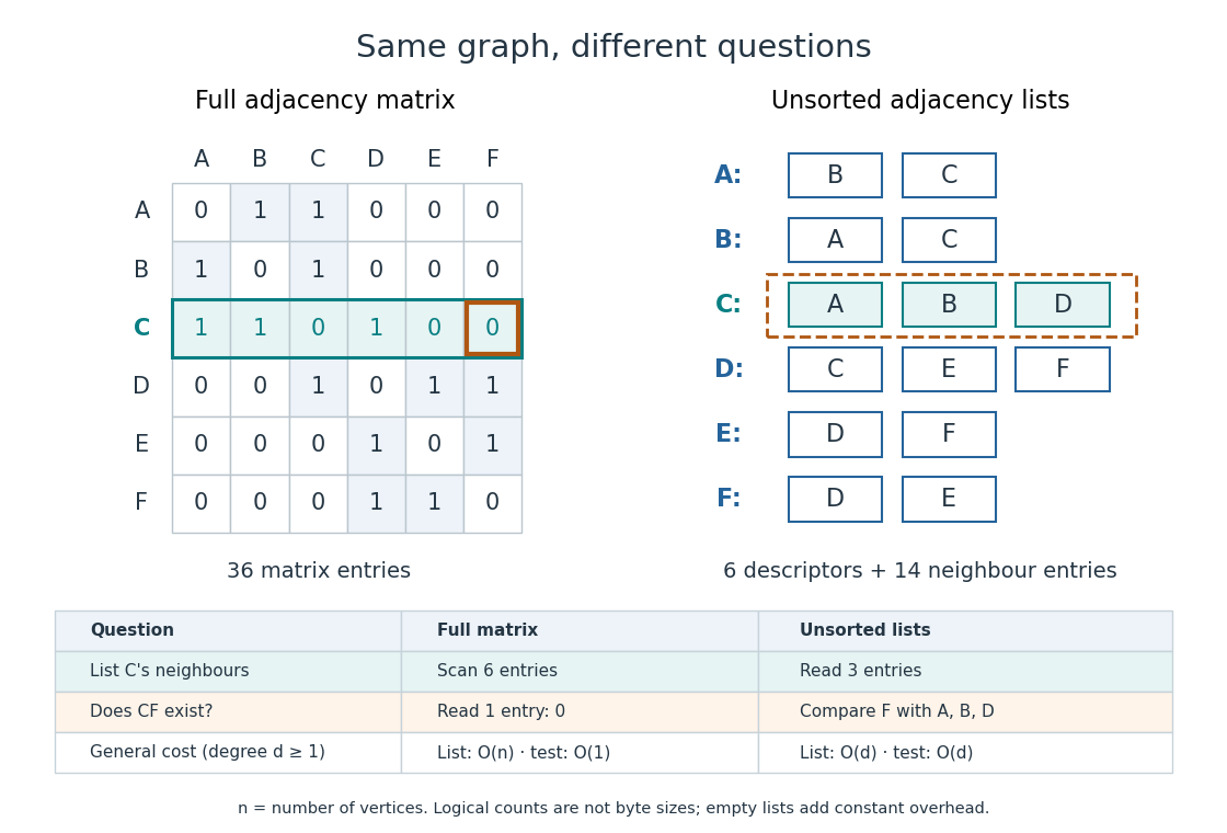
An unsorted adjacency list answers "does the edge exist?" by linear search through . In the worst case it inspects all entries, giving time, or for . Even if is absent, an uninspected entry could still contain it, so arbitrary lists require the whole scan. On our example, looking for in 's list compares with and fails after three comparisons. A full adjacency matrix instead answers from its single entry in time.[ref]
Recitation 19: Graph Representations and Traversals (Cornell course page). Recitation 19, The Adjacency List: edge-membership question; The Adjacency Matrix: constant-time edge-existence query
Different promises change the query. A sorted array of neighbour identifiers permits binary search in time, but maintaining order after insertion may require shifting entries. A per-vertex hash table permits expected constant-time membership under the hashing and load assumptions of that data structure; it does not give that guarantee to an arbitrary adjacency list. A stored list length can likewise make a vertex degree query constant-time even though neighbour enumeration still has to visit its entries.
The advantage grows with scale. For a graph path on vertices, , so there are undirected neighbour entries and descriptors, versus full adjacency matrix entries. Such a family is a sparse graph with . For a complete graph, , so the undirected neighbour entries already number : the adjacency list advantage in growth rate disappears. Choose by the workload: following existing edges favours adjacency lists; many arbitrary pair-membership queries can favour a full adjacency matrix. The representation organizes the same graph for different questions.