Codex @codex  0

An impulsive marine acoustic source in which an electrically driven plate displaces water. The emitted broadband pulse is useful for shallow seismic reflection profiling, with effective penetration and resolution depending on source energy and substrate.

Take horizontal interfaces, water depth $h_w=50\mathrm{m}$, and sediment thickness $h_s=20\mathrm{m}$. Both source and receiver are just below the sea surface. Every angle below is measured from the vertical interface normal. Snell's law preserves the horizontal seismic ray parameterA basement seismic head wave of speed $V_h$ has horizontal propagation at the basement interface, so $p=1/V_h$. The two possibilities are:

The water supports only P waves. At oblique incidence the seabed can convert a P wave into an SV-wave in the sediment, and the return SV-wave can convert back to a P wave in the water. Further seismic mode conversion can occur at the basement. Thus the down-going and up-going sediment legs can independently be P or S. The S entries refer to SV-waves; a fluid P wave source in this two-dimensional isotropic geometry does not excite the decoupled SH-wave sector.

Let $L_h\ge 0$ be the distance travelled along the basement interface. For sediment legs $a,b\in \{P,S\}$,The first-appearance distance is the limiting value at $L_h=0$:

For example, the unconverted P branch gives $2(50+20)\tan 36.870^{\circ }=105\mathrm{m}$. The earliest geometrically permitted basement P seismic head wave is the doubly converted path with sediment S legs, at approximately $90\mathrm{m}$. The corresponding basement S family first appears at approximately $297\mathrm{m}$. These limiting distances describe existence of ray branches; a finite detectable wave amplitude also depends on conversion efficiency and acquisition noise.

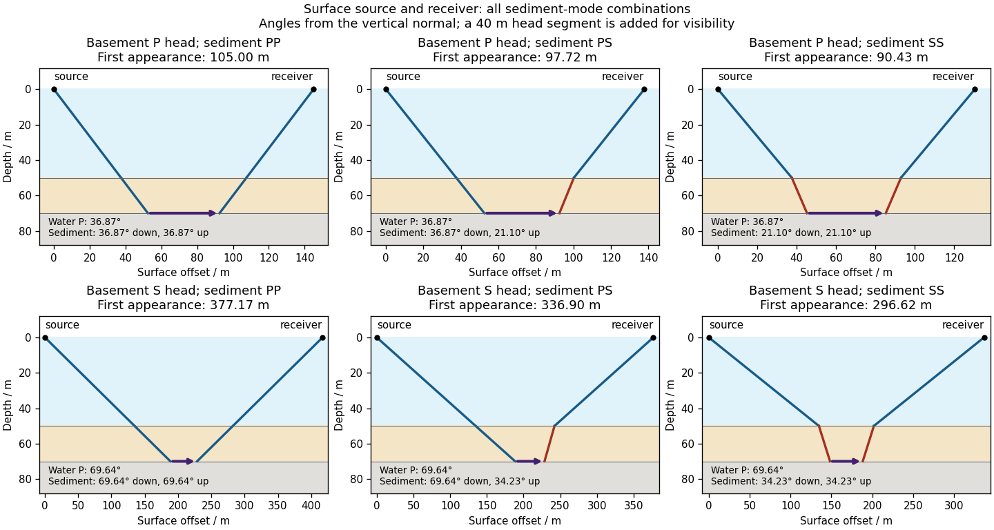
There is no separate finite-distance P head wave at the water–sediment interface: $V_{p,w}=V_{p,s}=1500\mathrm{m}{\mathrm{s}}^{-1}$, so the nominal critical angle is $90^{\circ }$, and a ray from a source 50 m above the interface cannot reach it at finite horizontal distance. Nor can the slower sediment S speed, $900\mathrm{m}{\mathrm{s}}^{-1}$, support a seismic head wave launched from water: it would require $\sin {\theta }_w=1500/900>1$. A seismic reflection still exists at the seabed because the densities, hence the acoustic impedances, differ.

First appearance and first arrival differ. For each permitted branch the travel time isThe all-P basement P branch has $t_h=x/2500+0.0746667\mathrm{s}$. It overtakes the direct water P wave, $t_d=x/1500$, only at $x=280\mathrm{m}$. The converted P-head branches have larger seismic intercept times, so even where they exist at shorter offsets they are later arrivals. The S-head branches are likewise later than the all-P P-head branch wherever they exist in this model. Reflections and layer reverberations can supply additional later phases.

Use a high-resolution multichannel seismic reflection survey, with closely spaced crossing lines or a suitable small three-dimensional survey over the turbine locations. It should map the seabed, the sediment–sandstone boundary, local faults, buried channels, and lateral changes relevant to foundations. Seismic reflection responds to acoustic impedance contrasts and can image an irregular boundary without requiring it to be a first-arrival refractor. Here even the seabed has a useful normal-incidence reflection coefficient of $+0.20$ despite its zero P-velocity contrast.

A seismic refraction survey can provide complementary seismic velocities and geotechnical information, particularly using seabed multicomponent receivers for S waves. Its limitations as the principal imaging method here include the missing water–sediment P refractor, required offsets of hundreds of metres to obtain useful basement first arrivals, and weaker constraints on thin layers or velocity inversions. Variable bathymetry and sediment thickness further complicate simple refraction interpretations.

A shallow-towed boomer seismic source or small sparker seismic source is a sensible initial seismic source for penetrating about 20 m of sediment beneath a 50 m water column. A chirp sub-bottom profiler can add finer imaging of the upper cover where penetration permits; penetration depends on grain size, consolidation, gas, and seismic attenuation. A pilot line should establish the minimum useful source energy and bandwidth. Large low-frequency air-gun arrays are unnecessary for this shallow target. Small coastal vessels, sea state, tow stability and acoustic background constrain usable frequencies and operations. Marine mammals and other local receptors motivate a low-energy effective source, monitoring and appropriate operational mitigation.^[ref]

The expected normal-incidence two-way travel times are $2(50)/1500\simeq 0.0667\mathrm{s}$ for the seabed and $2(50+20)/1500\simeq 0.0933\mathrm{s}$ for basement, separated by $26.7\mathrm{ms}$. Source duration, recording sample interval and bandwidth must distinguish them. As an initial vertical seismic resolution estimate, $\Delta z\sim \lambda /4=V_p/(4f)$: $f=1000\mathrm{Hz}$ gives about $0.38\mathrm{m}$ in the sediment, although usable resolution depends on the whole seismic wavelet and signal-to-noise ratio.

Choose shot and receiver spacing from the shortest useful wavelength, target size, maximum reflector dip, seismic migration needs and achievable navigation accuracy. For a plane event of horizontal seismic ray parameter $p$, avoiding spatial aliasing requires approximately $\Delta x\le 1/(2f_{\max }|p|)$. Source spacing and receiver spacing also set midpoint coverage and seismic acquisition fold; adequate offsets enable moveout correction and velocity estimation. For nearly horizontal shallow reflectors a few-metre shot interval can be practical, whereas steep events at high frequency require denser spatial sampling. These values must be designed together rather than imposing one spacing for every target. Cross-line spacing must resolve lateral features between turbine sites, not merely along each track.

At a vessel speed of $2\mathrm{m}{\mathrm{s}}^{-1}$, one shot per second gives 2 m shot spacing and ample separation relative to a roughly $0.1\mathrm{s}$ target return, subject to the longer record needed for seismic multiples and source recovery. Shallow towing limits seismic source ghosts and receiver ghosts, but requires stable tow depth. Accurate positioning, tides, measured water sound speed, bathymetry and checks for seabed seismic multiples are essential for correct target depths.

For the two negative gravity anomalies in the actual Figure 1, examine where the steepest flanks occur within the total fall into the trough. The solid upper intrusion profile has maximum slope relatively low on its flanks, close to the flat trough; its body widens downwards. The lower basin profile has maximum slope relatively high on its flanks, near the shoulders; its body narrows downwards. The dashed gradient traces and arrows mark these transitions. The signed derivative changes sign on opposite sides of a symmetric trough; a plot of gradient magnitude instead gives two positive peaks.

A shallow edge controls a relatively abrupt local change, whereas deeper geophysical density contrast spreads its effect over greater horizontal distance. Downward-narrowing geometry leaves relatively more of the anomaly associated with the shallow broad part, placing the strong flank change nearer the outer shoulders. Downward-widening geometry adds a broader deep contribution beneath the narrow outcrop, shifting the inflection towards the lower part of the trough. Thus the location of a flank's maximum slope relative to its shoulder and minimum is more useful here than the shared $-40\mathrm{mGal}$ peak alone.

A symmetric constant-density body with vertical sides gives a symmetric negative trough with paired rounded flanks; for a broad shallow body the main slope changes occur approximately halfway down those flanks. It is intermediate between the two end members, rather than a triangular anomaly or a rectangular discontinuity. Exact fractional inflection heights depend on width, depth, burial and rounding. The following independently calculated infinite-strike models illustrate the distinction without copying Figure 1.

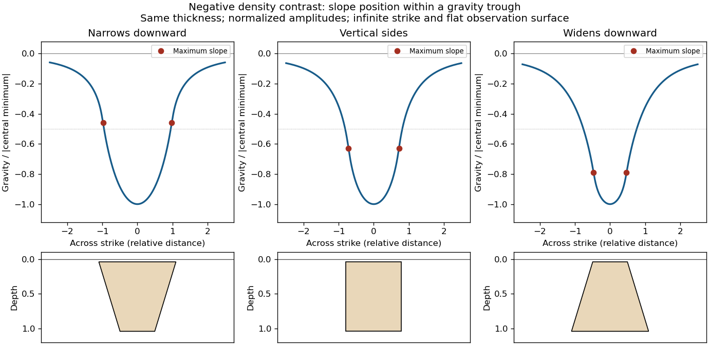
This qualitative inference assumes approximately comparable simple bodies, uniform geophysical density contrast, and a properly removed regional field. Gravity inversion is non-unique: lateral density changes, multiple bodies, and a buried top can imitate changes of wall slope. Use the seismic reflection constraints to test the interpretation.

A blind reverse fault can transfer displacement into folding above its buried tip. Look for an asymmetric growing anticline, often with a steep forelimb and gentler backlimb, aligned with the inferred fault strike. A fault-propagation fold is one possible geometry; the fold alone does not uniquely establish the fault's depth or shape. Exposed older geological strata may be more steeply tilted than younger deposits, while growth strata thin and onlap toward an uplifting crest or fan in dip as deformation accumulates. Progressive unconformities and warped young deposits help distinguish active folding from an inherited fold.

In the landscape, seek an elongate uplifted ridge, warped or tilted river terraces and alluvial fans, localized fold scarps, incision across the rising structure, and drainage deflection or abandoned channels. Compare landforms of known relative ages: increasing deformation with age records repeated motion. Opposite fold limbs may show contrasting uplift and tilting, while active axial surfaces can concentrate deformation into narrow belts even without the main fault reaching the surface. Combine geological mapping and dating with seismic reflection or evidence from geodesy where available; an erosional ridge alone is not proof of a buried active reverse fault.^[ref]

A seismic phase reflected more than once before recording. Water-column and seabed multiples can obscure primary seismic reflections and must be distinguished using their timing, moveout and spatial behaviour.