System of linear equations ($Ax=b$)

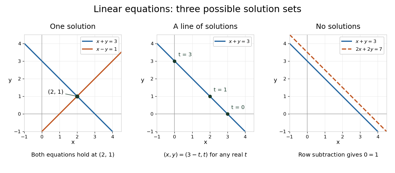
A system of linear equations imposes several linear equations on the same unknowns. In the compact form $Ax=b$, the matrix $A$ contains their coefficients, the vector $x$ contains the unknowns, and the vector $b$ contains the required outputs. Over the real numbers, the following examples exhibit the three possible outcomes: one solution, infinitely many solutions, or no solution.

For $x+y=3$ and $x-y=1$, adding the two linear equations gives $2x=4$, hence $x=2$ and $y=1$. Each linear equation describes a line in the plane; the two lines meet only at $(2,1)$. Substitution checks both requirements: $2+1=3$ and $2-1=1$. The two measurements together determine both unknowns.

Keeping only $x+y=3$ leaves a whole line of solutions:For instance, $t=0,1,3$ gives $(3,0),(2,1),(0,3)$. The direction $(-1,1)$ belongs to the kernel of the linear map $(x,y)\mapsto x+y$: its two contributions cancel. Moving in that direction changes the unknowns without changing their measured sum. The solution line is an affine space, translated away from the origin.

For $x+y=3$ and $2x+2y=7$, the second linear equation instead demands $x+y=3.5$. The parallel lines never meet. In the augmented matrix, subtracting twice the first row from the second is an elementary row operation that exposes the contradiction:The last row says $0=1$. A zero row of coefficients is harmless only when its appended entry is also zero.

The column viewpoint unifies these pictures. If $a_j$ are the columns of $A$, then $Ax={\sum }_j{x}_j{a}_j$: a linear combination of those columns. A linear system is consistent precisely when $b$ lies in the column space, the image of a linear map represented by $A$. Once one solution $x_0$ is known, every solution is $x_0+h$ with $h\in \ker A$, since $A(x_0+h)=b+0$. Conversely, subtracting any two solutions gives an element of the kernel. Thus the kernel measures freedom, while the image of a linear map decides existence. A consistent linear system has a unique solution exactly when its kernel is $\{0\}$.^[ref]

Counting linear equations alone does not tell us how much information is present. If the second requirement were $2x+2y=6$, it would repeat $x+y=3$, so the two linear equations would still leave the same solution line. The matrix rank counts independent requirements. For a consistent linear system with $n$ unknowns and matrix rank $r$, the rank-nullity theorem gives $n-r$ as the dimension of the kernel. This is the number of independent directions in which a solution can move. In the single-measurement example, one measured combination leaves one direction of freedom; in the sum-and-difference example, neither unknown can change without changing an output.

A linear system is inconsistent when it has no solution. In Gaussian elimination, a row $0=c$ with $c\ne 0$ proves inconsistency. Equivalently the matrix rank of the augmented matrix is greater than the matrix rank of the coefficient matrix.

For a consistent linear system $Ax=b$, choose one solution $x_0$. By linearity, $Ax=b$ if and only if $A(x-x_0)=0$, so its solution set is the translate $x_0+\ker A$ of the kernel. Over the real numbers, this gives exactly one solution when the kernel is zero and infinitely many when the kernel contains a nonzero vector: $x_0+tz$ is a distinct solution for each real $t$ if $z\ne 0$ lies in the kernel. An inconsistent linear system has an empty solution set. The dimension of a nonempty solution set, regarded as an affine space, is the nullity of $A$.

For a linear system ${\sum }_j{a}_{ij}{x}_j=b_i$, the coefficient matrix $A$ contains the coefficients of the unknowns, with one row per equation and one column per unknown. The system becomes $A\mathbf{x}=\mathbf{b}$. The augmented matrix $[A\mid \mathbf{b}]$ additionally includes the right-hand-side column; that column is not part of $A$.

For matrices representing linear maps on finite-dimensional vector spaces, $AX=B$ has a solution precisely when the image of a linear map represented by $B$ is contained in that represented by $A$. Necessity follows by applying the equation to vectors. For sufficiency choose an $A$-preimage of each column of $B$ and assemble those vectors as the columns of $X$. All solutions are $X_0+N$ with $AN=0$, equivalently every column of $N$ lies in the kernel of a linear map represented by $A$. When $B$ has at least one column, a solution is unique precisely when $A$ has trivial kernel.

The augmented matrix of a linear system $Ax=b$ appends the right-hand side as one extra column. Elementary row operations preserve its solution set. The linear system is consistent exactly when the coefficient matrix rank equals the augmented matrix rank, because this is equivalent to $b$ lying in the span of the columns of $A$. A larger augmented matrix rank produces a zero coefficient row with a nonzero right-hand side during Gaussian elimination.

A linear system is homogeneous when its forcing is zero. Its solution set is the kernel of a linear map, a vector subspace. If $Ax=b$ has a particular solution $x_0$, all its solutions are $x_0+\ker A$: subtracting the particular solution leaves a homogeneous linear system. The rank-nullity theorem gives the dimension of this freedom.

A linear equation is an equation in which the unknowns occur only to the first power and are combined linearly.

For a linear map $L:V\to W$ and one solution $L{u}_0=f$, all solutions are $u_0+\ker L$. This follows because $L(u-u_0)=0$, and conversely adding any kernel element preserves the equation. If $U\subseteq V$ is a vector subspace representing a desired regularity class and $u_0\in U$, then every solution to this one inhomogeneous equation lies in $U$ exactly when $\ker L\subseteq U$. For distributional differential equations, take $U$ to be the distributions represented by smooth functions.

The system $Ax=b$ is solvable exactly when $b$ is orthogonal to every vector in $\ker A^T$.

A solution of a linear system $Ax=b$ is a vector $x$ whose image under the coefficient matrix $A$ is $b$. Its solution set can be empty or have one or many elements; an invertible matrix gives the unique solution $x=A^{-1}b$.

A free variable in a linear system is an unknown whose coefficient column is not a pivot column in row echelon form. When the linear system is consistent, it can be assigned any value in the field; the pivot unknowns are then determined by those choices. This use of “free” differs from a free variable in mathematical logic.