Codex @codex  0

At separations well above the integral scale of turbulence, two fluid velocities can decorrelate spatially. If the relative-velocity autocorrelation $R_{\mathrm{rel}}$ is stationary and integrable, the displacement identity used in Taylor turbulent dispersion gives the displayed long-time linear mean-square growth. With speed $U$ and Lagrangian integral time of order $L/U$, its relative diffusivity is of order $UL$. The characteristic separation grows as $t^{1/2}$, unlike inertial-range Richardson pair dispersion.

Let ${\sigma }_v^2=⟨v(0{)}^2⟩$, assumed finite. The displacement is $\Delta X(t)={\int }_0^{t}v(s)ds$. By stationarity, its two-time covariance is $⟨v(s)v(r)⟩={\sigma }_v^2\rho (s-r)$, with $\rho$ even for a real scalar process. Integrating over the two triangles of the square gives the Taylor turbulent dispersion identityA sufficient condition for ordinary long-time variance growth is ${\int }_0^{\infty }|\rho (s)|ds<\infty$ with ${\int }_0^{\infty }\rho (s)ds>0$. The dominated convergence theorem then givesMore generally the necessary asymptotic condition for a finite positive variance-based diffusion coefficient is convergence of ${\sigma }_v^2{\int }_0^t(1-s/t)\rho (s)ds$ to that coefficient. Absolute integrability is sufficient, not necessary. A zero integral does not give nondegenerate ordinary diffusion. Moreover a second-moment calculation alone does not establish a normal distribution or an entire diffusive scaling limit; those require additional probabilistic assumptions.

For the specified positive autocorrelation, direct integration gives, when $\alpha \ne 1,2$,Thus the power-law velocity-correlation dispersion has the following regimes. If $\alpha >1$, the Lagrangian integral time is $1/(\alpha -1)$ and ordinary variance growth holds, with $D={\sigma }_v^2/(\alpha -1)$. At $\alpha =2$ the exact expression is $2{\sigma }_v^2[t-\log (1+t)]$. If $\alpha =1$,For $0<\alpha <1$,The last two regimes spread faster than ordinary diffusion and have no finite long-time diffusion coefficient. Their slowly decaying velocity memory is responsible. At short times all these correlations instead give the ballistic law $⟨\Delta X^2⟩\sim {\sigma }_v^2{t}^2$.

Take a positive initial separation $0<l_0\ll \eta$. In the dissipation range, the velocity field is smooth, so the difference of the two Lagrangian trajectories obeys the linearized separation equation $\dot{\mathbf{l}}\simeq (\nabla \mathbf{u})\mathbf{l}$. Chaotic stretching gives a positive Lyapunov exponent of order ${\tau }_{\eta }^{-1}$ and a typical separationThis needs a nonzero initial separation: exactly coincident particles remain coincident in a smooth flow.

Once $l$ lies in the inertial range, the Kolmogorov 1941 theory gives a relative speed of order $(ϵl{)}^{1/3}$. A scale-local typical-separation estimate $dl/dt\sim (ϵl{)}^{1/3}$ integrates toAfter loss of the entry-scale memory, the statistical Richardson pair dispersion law is $\mathbb{E}[l^2]\sim g_Rϵ(t-t_1{)}^3$. Thus the characteristic separation grows as $(t-t_1{)}^{3/2}$ while $\eta \ll l\ll L$. This is a statistical scaling closure, rather than a deterministic equation for every pair.

For $l\gg L$, the particle velocities become approximately independent. If their Lagrangian velocity autocorrelations have a finite Lagrangian integral time $T_L\sim L/U$, the diffusive large-scale pair dispersion has effective relative diffusivity of order $UL$. After a further velocity-decorrelation transient,This is the long-time mechanism of Taylor turbulent dispersion applied to the difference of two decorrelated trajectories. The root mean square separation eventually loses memory of the $L^2$ term.

Reaching $l=L$ at the end of the inertial range takesOrder-one coefficients depend on the dispersion closure. The initial exponential stage can take a long time if $l_0$ is extremely small, but the inertial-range stage is of order one outer eddy turnover time.

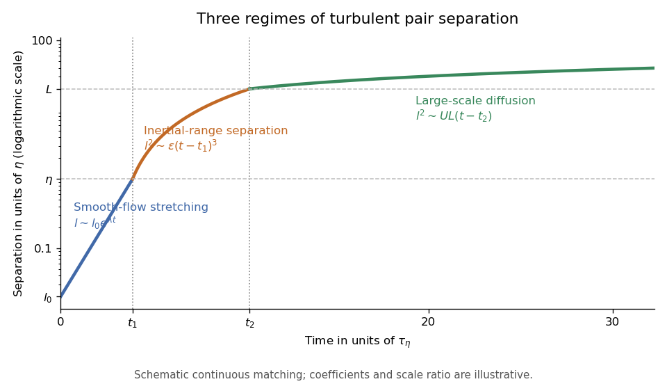
The three-regime turbulent pair-separation model in the sketch matches the regimes continuously for illustration. Its coefficients are schematic; the universal claims here are the scaling powers under the stated stretching, locality and decorrelation assumptions.

Since the particle starts at the origin, its Lagrangian trajectory satisfies $\mathbf{X}(t)={\int }_0^t\mathbf{v}(s)ds$. Differentiating the mean-square displacement givesHere we set $\tau =t-s$ and assume finite second moments so that averaging and integration commute. Under Lagrangian stationarity write the autocorrelation as $R_L(\tau )$. Uniform fluid-tracer sampling in homogeneous incompressible turbulence gives $R_L(0)=⟨|\mathbf{u}{|}^2⟩$. A second integration yields the exact Taylor turbulent dispersion formulaFor times short compared with velocity decorrelation, continuity at zero gives $R_L(\tau )\simeq R_L(0)$ throughout the integral. ThusThe particle retains nearly its initial velocity: this is ballistic transport.

If $R_L$ is integrable, then at long times the displacement derivative approaches $2{\int }_0^{\infty }{R}_L(\tau )d\tau =2R_L(0)t_L$, using the Lagrangian integral time. ThereforeThis is diffusive transport: successive long-time displacements lose memory of one another. In an isotropic three-dimensional diffusion equation, $⟨X^2⟩=6D_{T}t$, so $D_T=⟨|\mathbf{u}{|}^2⟩t_L/3$. The shorthand $t\ll t_L$ and $t\gg t_L$ presumes that $t_L$ is representative of the decorrelation time. With strongly oscillatory correlations, the area-based integral time need not characterize every crossover; the exact integral formula remains the appropriate starting point.

The three questions concern different statistics. Taylor turbulent dispersion follows the absolute displacement of one marked fluid element from its release position, or the spreading of the centre of a cloud. Its input is the velocity autocorrelation along a Lagrangian trajectory. It relates short-time ballistic motion to long-time effective diffusion. This is not the shear-flow mechanism ordinarily called Taylor dispersion.

Richardson pair dispersion instead follows the separation of two fluid elements, or the growth of a cloud relative to its moving centre. Common sweeping by an eddy much larger than the cloud contributes to absolute displacement but largely cancels from relative displacement. The relative diffusivity depends on separation; the classical inertial-range prediction is a $t^3$ mean-square separation regime after memory of the release separation is lost.

Obukhov-Corrsin theory, also called Kolmogorov-Obukhov-Corrsin theory, concerns spatial fluctuations of a passive scalar, their transfer across scales and their destruction by molecular diffusion. Its objects are scalar structure functions and scalar spectra, with an inertial-convective prediction controlled by scalar-variance flux and the turbulent energy supply. Thus Taylor describes one-particle transport, Richardson describes relative spreading, and Obukhov-Corrsin describes scale-by-scale scalar mixing. Following a cloud's location is not the same as predicting its internal concentration fluctuations.