Codex @codex  0

For a finite-state homogeneous continuous-time Markov chain with transition intensity matrix $Q$, integrate the indicator of occupying state $j$ over $[0,T]$. Interchanging the bounded time integral and expected value gives the displayed integral of transition probabilities. It counts all visits, not only the first holding time. Summing over states gives $T$. A zero eigenvalue of $Q$ does not cause a problem for this integral, although it prevents casually writing it with an inverse matrix $Q^{-1}$.

An irreversible three-state illness-death model allows progression $1\to 2$ and death $1\to 3$ or $2\to 3$, with state 3 absorbing. A constant-rate transition intensity matrix uses three free rates $a,b,c$ and rows $(-(a+b),a,b)$, $(0,-c,c)$ and $(0,0,0)$. The labels can represent disease severity rather than literal health versus illness.

Use the compartment counts $Z_n=(S_n,I_n,R_n)$ as the state of the SIRS Markov chain. Its state space is $\{(S,I,R)\in {\mathbb{Z}}_{\ge 0}^3:S+I+R=n\}$. The transition rates areEach susceptible has infection hazard $\lambda I/n$, so summing over the $S$ susceptibles gives the first rate. The memorylessness of the exponential distribution makes each of the $I$ current infectives have recovery hazard $\gamma$, irrespective of its infection time. Each removed individual has immunity-loss hazard $\nu$. These are all the possible off-diagonal transitions. The diagonal entry of the transition intensity matrix is minus their sum, and a transition with no eligible individual has rate zero. Thus the three total event rates are $\lambda SI/n$, $\gamma I$ and $\nu R$, and every event conserves population size.

Let $q_{rs}$ be the transition intensity from state $r$ to $s$, and let $Q$ be the transition intensity matrix, with $q_{rr}=-{\sum }_{s\ne r}{q}_{rs}$. For a continuous-time multi-state model with the time-homogeneous Markov property, the transition probability matrix is $P(u)=e^{uQ}$, with entry $p_{rs}(u)$. Condition on each recorded initial state. Panel visits contribute transition probabilities; an exact entry into the absorbing death state contributes a statistical probability densityThis mixed panel and exact-death likelihood sums over the living state just before death. It accounts for survival until the event; replacing its final factor by $p_{r3}(u)$ would count deaths throughout the interval.

Using the actual visit times recovered from the PDF, the three individual likelihood contributions areHere $g_{23}$ means $g_{r3}$ with $r=2$, not a transition probability. Subjects 8 and 9 supply no event-density factor after their last panel observation. Assume independent subjects and noninformative examination and censoring times; conditional on their observation schedule, its distribution supplies no additional statistical parameter-dependent factor. The patients' covariates can be incorporated by using their own $Q_i$ in these same expressions.

For the progressive structure used in the subsequent output, put $a=q_{12}$, $b=q_{13}$, $c=q_{23}$ and $\lambda =a+b$. The progressive illness-death model permits no recovery, soWhen $\lambda =c$, the continuous limit is $p_{12}(u)=au{e}^{-cu}$. Thus the likelihood contributions simplify toIntermediate unobserved disease transitions remain integrated into each panel transition probability.

Let $z_i=(S_i,E_i,A_i{)}^T$ contain sex, the education indicator, and age at diagnosis. Write $\overline{z}$ for the sample means. The output's baseline transition intensities are evaluated at those means, so use the centred log-linear transition intensity modelThe full transition intensity matrix isThe fitted centred baselines are $(q_{12},q_{13},q_{23})(\overline{z})=(0.1821,0.0126,0.0450)$, and fitted slope vectors in sex–education–age order areThe two sex coefficients displayed as zero are fixed by the specified constraints; they are not estimated to be exactly zero. There are three free baseline transition intensities and seven free covariate slopes. The sample means are not printed, so uncentred intercepts at $z=0$ cannot be recovered numerically from this output.

Conditional on fixed covariates, subjects follow independent, correctly classified continuous-time multi-state models obeying the time-homogeneous Markov property, with $P_i(u)=e^{u{Q}_i}$. The progression is irreversible and death absorbing, with constant transition intensities during follow-up for each subject. In particular, the model uses fixed age at diagnosis rather than attained age. It assumes noninformative observation and censoring, and treats death times as exact through the mixed panel and exact-death likelihood. The Markov property rules out an additional effect of elapsed time in the current state after conditioning on it and the recorded predictors.

There are three free transition intensities: progression, death from the initial state, and death from the advanced state. In the three-state illness-death model, state 3 is an absorbing state, and there is no recovery transition.

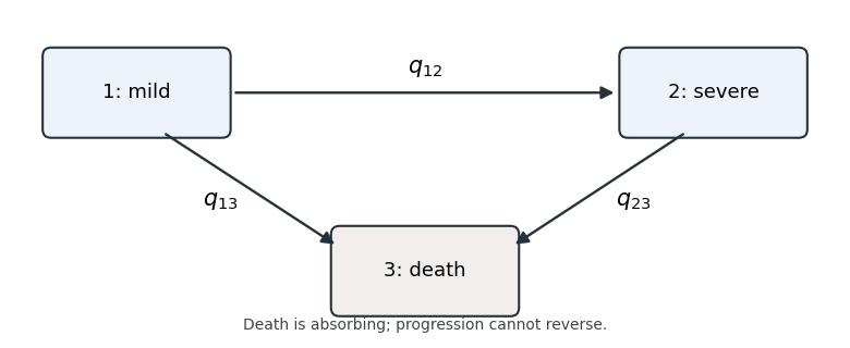
Writing $a=q_{12}$, $b=q_{13}$ and $c=q_{23}$, with all three nonnegative, the transition intensity matrix isEach diagonal entry is minus the sum of the row's outgoing transition intensities, rather than an additional unknown parameter. A continuous-time multi-state model with these rates describes the severity labels in the observations; an explicit cured state would require a richer state space.

For a finite-state continuous-time Markov chain, a transition intensity matrix has nonnegative off-diagonal rates $q_{rs}$ and $q_{rr}=-{\sum }_{s\ne r}{q}_{rs}$. Every row sums to zero. In the time-homogeneous case its transition probability matrix is the matrix exponential $P(t)=e^{tQ}$. An absorbing state has a zero row.