Codex @codex  0

Retain $a=p_0^{1/\gamma }/{\rho }_0$ from part (b), and use time translation invariance to write $G(\mathbf{x},t;\mathbf{y},\tau )=g(\mathbf{x},\mathbf{y};t-\tau )$. Define the temporal Fourier transform byMultiplying the transformed Green function equation by $-a(\mathbf{x})$ givesThis is a symmetric divergence-form spatial operator, although the original unweighted operator need not be symmetric in the ordinary volume measure.

Let $G_j(\mathbf{x})=\tilde{G}(\mathbf{x},{\mathbf{y}}_j;\omega )$. The product rule gives the bilinear Green second identityThe frequency terms cancel. Integrating over the domain, the right side becomesThe boundary integral is zero for common homogeneous Dirichlet boundary condition, Neumann boundary condition or reciprocal Robin boundary condition conditions. In an unbounded domain, use the same outgoing limiting-absorption prescription for both Green functions; it gives the corresponding vanishing boundary pairing. This identity has no complex conjugation: it proves transpose wave reciprocity, not a Hermitian or time-reversal identity. We obtain the weighted acoustic Green-function reciprocityThe factor is frequency independent, so inverse Fourier transform gives the same relation at equal time lag. Both time arguments below have lag $t-{\tau }_2$, henceReciprocity exchanges source and receiver while preserving elapsed time; it does not turn a causal response into an advanced one.

In time reversal acoustics, the array records the incoming signal, reverses each recorded time trace, and re-emits it through the same medium. This is phase conjugation in the frequency domain. For the time-harmonic wave convention $e^{-i\omega t}$, reversing a real time trace replaces its positive-frequency wave amplitude by its complex conjugate. The medium must remain unchanged between recording and re-emission.

Let $f(\mathbf{z})={\Psi }_0(0,\mathbf{z})$ and $G_L(\mathbf{\zeta },\mathbf{z})=G(L,\mathbf{\zeta };0,\mathbf{z})$, with the chosen source and array normalizations incorporated into the Green function. Let $a(\mathbf{\zeta })\ge 0$ be the array's aperture weight, equal to the indicator of its receiving region for an ideal uniform array. The recorded field isBy wave reciprocity, back-propagation has the same Green function with the source and receiver exchanged. Therefore the physically re-emitted, back-propagated wave amplitude isIf $Hf=R$ and $P_A$ multiplies by $a$, then ${\Psi }_B=H^T{P}_A\overline{Hf}$, where $T$ denotes the transpose without conjugation. Taking a final complex conjugate instead defines the adjoint reconstruction $\overline{{\Psi }_B}=H^{\ast }{P}_{A}Hf$. This distinction prevents an erroneous conjugation in the time reversal operator.

For a localized Gaussian beam or acoustic point source in a homogeneous medium, a finite aperture admits a limited range of angles. The focal width is of order $\lambda L/A$ when $A$ denotes the aperture diameter. In a random medium, multiple scattering creates paths with a larger angular spread. Each reversed path retraces its route, and the paths interfere constructively at the source. This can produce a larger effective aperture in time reversal and a narrower focus, even though the unreversed field has a complicated speckle pattern.

This comparison concerns a homogeneous reference medium; a deterministic heterogeneous medium can also provide useful multipath propagation. Suitable scale limits or frequency and spatial averaging can make refocusing self-averaging. Such self-averaging is not automatic for every monochromatic source and every random realization. Wave absorption, changing medium parameters, unresolved paths or poor array coverage can spoil refocusing. With complete capture of the propagating modes and a lossless unitary operator $H$, ideal adjoint reconstruction is already exact in either medium. Random scattering can improve finite-aperture wave focusing through angular diversity. See the regime-dependent analysis in Statistical stability in time reversal.

To first order in $n_{ϵ}$, replace $q$ by $2n_{ϵ}$ and use the known incident field in the outgoing integral. The Born approximation for scalar wave scattering givesBoth the $n_{ϵ}^2$ contrast term and the internal-field correction are second order for fixed geometry in the perturbative regime established in part i.

Specify the data space before taking an adjoint operator. For example, let $X=L^2(B)$ and $Y=L^2(\Gamma )$, where $\Gamma$ is a bounded measurement surface separated from $B$. Define the linear operatorFor bounded incident field this is a Hilbert-Schmidt operator, hence a compact operator. The equation is $A{n}_{ϵ}=y$, with $y={\psi }_s{|}_{\Gamma }$. Other sampling geometries give corresponding data spaces and weights; the paper does not specify one. Using the usual complex $L^2$ inner products, its adjoint operator isThe complex conjugations are required by the adjoint operator identity, not by wave reciprocity alone.

The Landweber iteration starts from $f_0=0$ and applies gradient descent to $\frac{1}{2}\Vert Af-y{\Vert }^2$:Each step back-propagates the data residual. The Landweber relaxation parameter controls stability, and early stopping of Landweber iteration prevents small singular values from amplifying measurement errors. For an explicitly real-valued index contrast, use the real Hilbert space structure and replace $A^{\ast }$ by $\mathrm{Re}{A}^{\ast }$ in this update. Additional sign or support constraints require corresponding projections; none are assumed here.

Consider an optical point source at $(z,x)=(0,0)$, a uniform transparent medium, and a flat return surface $z=L$. A light ray with slope $s$ reaches $(L,sL)$. A phase-conjugate mirror reverses its full direction and returns it to $(0,0)$. An ordinary mirror reverses only its normal direction; its returning light ray reaches $x=2sL$ at $z=0$. Thus rays with $s=-1/4,0,1/4$ at $L=3$ return to $x=-3/2,0,3/2$ with ordinary specular reflection, but all return to $x=0$ under ideal phase conjugation. These are stipulated geometric coordinates, not laboratory measurements.

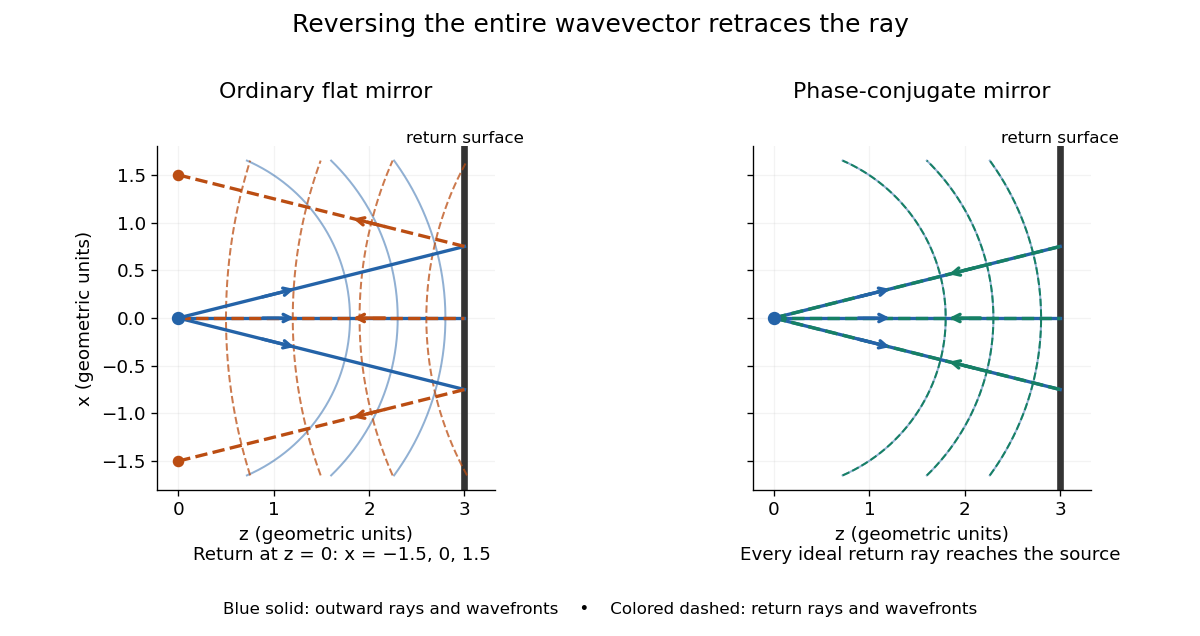
Solid blue curves mark outward wavefronts; dashed curves mark returning wavefronts. In the phase-conjugate mirror panel the returning curves coincide with the outward ones, and the arrows reverse on the same light rays. The diagram uses equal spatial scales. In geometrical optics, reversing each light ray in an unchanged medium with wave reciprocity retraces its route. At the optical point source itself, the ray construction becomes singular and diffraction sets the physical focal size.

A wave-level proof outline applies to a stationary scalar medium with real refractive index $n(\mathbf{r})$ and no wave absorption. Writing $c$ for the vacuum speed of light, its Helmholtz equation isAll coefficients are real, so complex conjugation gives the same Helmholtz equation for $U^{\ast }$. The conjugated outgoing boundary data select the incoming solution. This explains the connection between phase conjugation and retracing, provided the required incoming field is supplied over the necessary aperture. It also exposes the limits: wave reciprocity alone does not imply absence of wave absorption; conjugation of complex material coefficients would describe a different medium. Loss, an incomplete aperture, a changing medium or failure of wave reciprocity can prevent exact reconstruction. Intensity-dependent material changes need a separate analysis and are not covered by this linear proof.