A fundamental Gaussian beam is an ideal beam of light whose transverse wave amplitude has a Gaussian function profile. Here consider a circularly symmetric beam in vacuum, with propagation along , two transverse coordinates , and radius from the optical axis. With the beam waist at , total power , and vacuum wavelength , its time-averaged light intensity, meaning irradiance in , isHere is the minimum beam radius, and is the Rayleigh range. Far from the beam waist, with beam divergence half-angle . These are the fundamental circular Gaussian beam laws within the scalar paraxial approximation, appropriate when and the beam divergence is small. The underlying envelope solves the parabolic wave equation exactly; this does not make it an exact vector solution of Maxwell equations. [ref].
The radius convention matters. Writing for the complex wave amplitude envelope, the same is the wave amplitude radius and the light intensity radius:At these ratios are and , respectively. The light intensity radius is instead . None of these radii is a sharp edge: the ideal Gaussian function has nonzero tails at every finite radius. Kogelnik and Li explicitly use the wave amplitude radius in their fundamental-mode treatment. [ref]
https://dielslab.unm.edu/sites/default/files/Kogelnik66_0.pdf. Herwig Kogelnik and Tingye Li, Laser Beams and Resonators, Applied Optics 5, 1550–1567, 1966, §3.2
.For a numerical example, take vacuum wavelength and beam waist radius . Substitution gives Rayleigh range and far-field beam divergence half-angle . At , the beam radius is and the on-axis irradiance is half its waist value. At the same wavelength, halving the beam waist radius to quarters the Rayleigh range to and doubles the beam divergence half-angle to . At fixed power, that smaller beam waist also quadruples the peak irradiance.
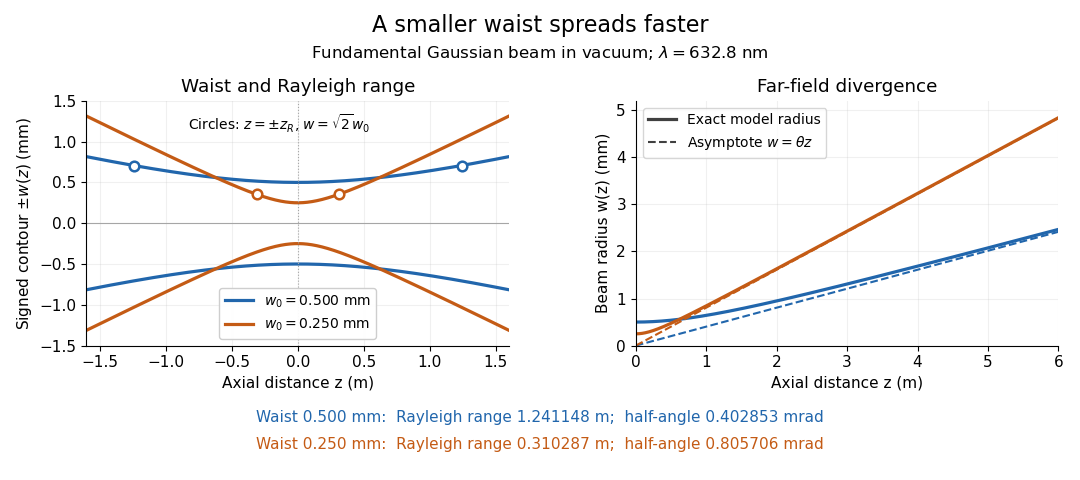
Gaussian beam radii at 632.8 nm: a smaller beam waist gives a shorter Rayleigh range and greater beam divergence
. Details. The contours in the left panel are in a plane through the optical axis; they mark an light intensity level, not an outer boundary. The right panel compares the exact model radii with the far-field asymptotes . The horizontal and vertical axes use different length units, so the drawn slopes are not physical angles.
The normalization expresses conserved power during free propagation. In transverse polar coordinates, an annulus has area , soA proof outline is the substitution in this integral. Spreading reduces peak irradiance as while increasing transverse area as , leaving power unchanged. In particular, the disk of radius contains , or , of the total power; the local light intensity at its rim is only of the on-axis light intensity. These are different quantities.
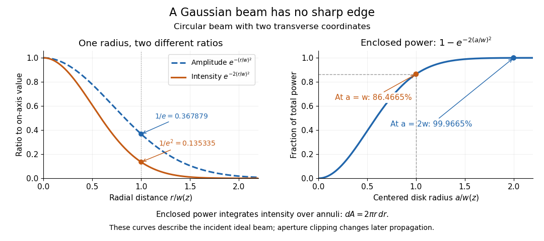
The left panel compares normalized wave amplitude magnitude and irradiance; the right panel integrates the transverse area to show enclosed power. For an ideal absorbing circular aperture of radius centered on the optical axis, the same fraction gives the power passing the aperture at that plane. An aperture of radius clips about of the incident power; radius clips only , or . After clipping, extra diffraction means the transmitted field no longer obeys the unmodified ideal Gaussian beam law. Every finite aperture cuts some ideal tail. Kogelnik and Li distinguish their large-aperture beam analysis from their finite-aperture diffraction analysis. [ref]
https://dielslab.unm.edu/sites/default/files/Kogelnik66_0.pdf. Kogelnik and Li, 1966, §§3–4
.The useful tradeoff is that a small bright spot cannot remain narrow indefinitely. An optical lens can create a smaller beam waist, but diffraction then makes the beam spread faster. The particularly simple relation ties localization directly to beam divergence. A proof outline for the propagation law starts with . The parabolic wave equation separates into two transverse factors, and a Gaussian integral in each coordinate givesHere is dimensionless and is the wavenumber; the carrier convention is , with angular frequency . Taking the squared complex modulus gives the stated and its light intensity scaling. Each transverse factor contributes , explaining the prefactor here and the different prefactor in the preserved Gaussian beam with one transverse coordinate.
Historically, Gaussian beam theory developed alongside early laser resonator theory and lens-guided transmission. In their 1966 review, Kogelnik and Li credit Boyd and Gordon, and Goubau and Schwering, with early beam treatments; they summarize earlier work rather than claim the whole construction as a new discovery. Their paper brings beam propagation, focusing and finite-aperture diffraction into a common practical account. [ref]
https://dielslab.unm.edu/sites/default/files/Kogelnik66_0.pdf. Kogelnik and Li, 1966, introduction and §3
.Fourier localization of a Gaussian beam expresses the tradeoff between a narrow transverse field and a broad distribution of transverse spatial frequencies. At a waist, takeTwo Gaussian integrals giveReducing therefore broadens the angular spectrum method representation rather than merely shrinking a picture in the same set of propagation directions.[ref]
Physical origin of the Gouy phase shift by Simin Feng and Herbert G. Winful. Equations 4–12, transverse confinement, spectral description and Gaussian phase
Widths must state their weighting. Normalize and to define transverse position and transverse-wavenumber distributions. Their one-coordinate standard deviations areThese are optical field-width statements under the stated Fourier convention, not an inference that each ray has simultaneously measured position and angle. Using amplitude widths instead would give different numerical factors.
For a strongly paraxial spectrum, and . The usual far-field Gaussian light intensity half-angle is . For original nm and mm, mm and mrad; the conventional divergence half-angle is about 0.4029 mrad. Halving the waist doubles both angular measures.
An illustrative apparatus places a camera in a plane conjugate to the waist and another measurement at a lens's back focal plane, where transverse spatial frequency maps to position in the paraxial model. Comparing widths tests localization and angular spread, provided magnification, focal length and detector response are accounted for. Finite aperture clipping changes the field and produces extra spectral structure, so the exact Gaussian width product cannot simply be assigned to every clipped beam.
The same spectrum also bounds the paraxial approximation: keeps most amplitude at transverse wavenumbers much smaller than . Strong focusing can require vector polarization constraints and a nonparaxial propagation model.
The Gouy phase describes the additional axial phase associated with a focused wave relative to a plane wave. For a fundamental circular Gaussian beam with beam waist at and Rayleigh range , defineWith the carrier convention , the on-axis field phase is up to a constant. Thus the signed additional phase is in this convention; defining the positive function does not reverse the physical prediction.[ref]
Physical origin of the Gouy phase shift by Simin Feng and Herbert G. Winful. Equation12, printed p.486, sign convention for the Gaussian phase contribution
The complex field prefactor gives a short derivation. The normalized Gaussian propagation factor isIts modulus describes the on-axis amplitude reduction; its argument is the additional phase. An intensity measurement alone loses this argument, so measuring the beam's width and brightness does not directly measure the Gouy phase.
As runs from far before to far after the waist, runs continuously from to . The total additional phase change has magnitude , but is not a discontinuous jump at the waist. For stipulated and , . Between and , the additional phase changes by ; the far-field-to-far-field limit gives .
The number of confined transverse directions matters. A Gaussian beam with one transverse coordinate has prefactor and half this phase contribution. Simin Feng and Herbert G. Winful's primary analysis relates the effect to transverse confinement and the angular spectrum representation: a localized beam includes transverse wave-vector components, affecting axial propagation.[ref]
Physical origin of the Gouy phase shift by Simin Feng and Herbert G. Winful. Equations4–12 and line-focus versus point-focus discussion, pp.485–486
An illustrative Gouy phase interferometry experiment overlaps the focused beam with a coherent reference beam and records the interference phase at different axial planes. Removing the ordinary optical-path contribution and accounting for wavefront curvature isolates the axial phase change. This is a proposed measurement outline, not an experimental result reported by the cited theoretical paper. In an optical cavity, related phase contributions help determine the resonance condition and distinguish transverse modes.
Gouy phase interferometry compares a focused field with a coherent reference to recover the additional Gouy phase. Beam brightness alone discards the phase. An interferometer converts a relative field phase into intensity modulation, but the optical paths and reference wavefront curvature must be modeled.
A published 2023 experiment by Lyubomir Stoyanov and colleagues used a Mach-Zehnder interferometer to study Bessel-Gaussian beams. Its setup included a 532-nanometre laser, beam expansion, two spatial light modulators, focusing lenses and a CCD camera on a rail to follow propagation after the focus. Its Figure 3 also describes a single-lens interferometer arrangement for stronger focusing.[ref]
Gouy phase of Bessel-Gaussian beams: theory vs. experiment by Lyubomir Stoyanov and others. Figure 3, printed p. 13691, apparatus caption
Structured modes need their own phase model; that experiment should not be silently interpreted as a fundamental-Gaussian measurement.A separate original protocol illustrates four-step phase retrieval. At one detector point, apply controlled signal-arm phases while the beam intensities remain fixed. Write
This phase-shifting interferometry formula removes the unknown common intensity background and positive modulation amplitude . It returns phase modulo ; phase unwrapping requires continuity information between sampled positions. If the interference visibility vanishes, the phase is not observable by this formula.
This phase-shifting interferometry formula removes the unknown common intensity background and positive modulation amplitude . It returns phase modulo ; phase unwrapping requires continuity information between sampled positions. If the interference visibility vanishes, the phase is not observable by this formula.
For a synthetic coherent Gaussian/reference pair, use reference intensity 1 and signal intensity , with . Then , and after common path phases are removed. At , the four intensities are , giving . At , the first intensity is still , but the quadratures reverse and the retrieved phase is .
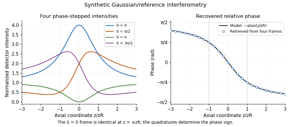
Original synthetic four-step interferometry of a Gaussian beam: symmetric single-frame readings become distinguishable through phase quadratures. No experimental data are shown.
Details. Curvature bias in Gouy-phase measurements is important away from the axis: the signal adds to its spatial phase. Fit or remove that term when using multiple pixels, retain calibrated phase steps and account for drift between frames. The recovered phase combines all coherent optical-path contributions until those controls isolate the Gouy phase.
Curvature bias in Gouy-phase measurements occurs when a spatially varying wavefront-curvature wave phase is mistaken for the axial Gouy phase in an interferometric comparison. For a fundamental Gaussian beam with time convention , the signal wave phase containsA curved reference contributes its own quadratic wave phase. After subtracting common axial path terms, the measured relative wave phase isThus a phase-retrieval algorithm can work exactly while the subsequent physical interpretation is biased. The Gaussian confinement wave phase and its arctangent dependence are derived in the primary theoretical treatment.[ref]
Physical origin of the Gouy phase shift by Simin Feng and Herbert G. Winful. Equations 4–12, Gaussian field phase and confinement
For an original example with a planar reference and stable path wave phase, let and . At and fixed detector radius , the curvature term is 0.5 radians. The true axial contribution is , whereas that off-axis pixel gives radians. At the curvature term reverses. Comparing those two axial planes at this fixed radius gives a wave phase change , differing from the axial Gouy change by one radian.
The effect is observable even where the signal is appreciable: at , is inside the plane's Gaussian radius . Avoiding only dim pixels does not remove curvature bias.
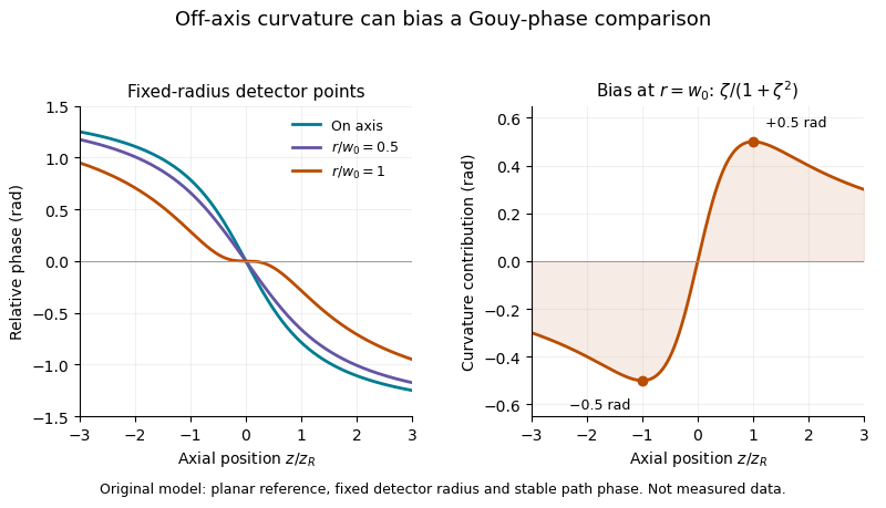
A useful measurement fits the spatial quadratic wave phase, identifies the beam center and reference curvature, and extrapolates the relative wave phase to the axis. Tilt, decentering and path drift require their own terms; averaging several pixel phases is not automatically equivalent to measuring the on-axis wave phase. Phase unwrapping can be required before fitting a wave phase profile.
The primary 2023 Bessel-Gaussian experiment documents focusing optics and a rail-mounted camera in its interferometer.[ref]
Gouy phase of Bessel-Gaussian beams: theory vs. experiment by Lyubomir Stoyanov and others. Figure 3, p. 13691
It motivates tracking both propagation position and wavefront geometry, but its structured-mode observations must not be silently reclassified as measurements of the illustrative fundamental-Gaussian model above.For a circular Gaussian beam with intensity proportional to , the displayed is the intensity radius. Its minimum is the beam waist radius, while the larger radius at a cavity mirror is not itself a waist. The Rayleigh range is .
The complex beam parameter combines a Gaussian beam's wavefront curvature and spot radius : . With , the beam waist is . A real paraxial ray transfer matrix maps it by . Positive imaginary part selects the physical finite-width branch in this convention.
A real paraxial ray matrix transforms a Gaussian beam parameter by the displayed fractional-linear map. For a lossless round trip with determinant one, a fixed point with positive imaginary part generically requires . Scalar matrices are degenerate exceptions: their fractional-linear map fixes every physical beam parameter even at the boundary. Finite apertures and resonance phases impose additional physical constraints.
The beam waist is the narrowest cross-section of a freely propagating Gaussian beam. Its radius uses the wave amplitude , or light intensity , convention; its diameter is . Specifying a “spot size” without saying radius or diameter can introduce a factor-of-two error. Within the scalar paraxial approximation, the wavefront at the beam waist is planar. The minimum radius sets both the Rayleigh range and the far-field beam divergence.
The Rayleigh range of a fundamental Gaussian beam in vacuum is the positive axial distance from the beam waist at which its radius grows from to . Thus its contour area doubles and its peak irradiance halves. Within , the radius stays at most ; for , beam divergence dominates. At fixed vacuum wavelength, the Rayleigh range scales quadratically with the beam waist radius. The formula here uses the vacuum wavelength, not an unlabelled wavelength in a material.
For the free parabolic wave equation , input with propagates asThe branch is continuous from . One-dimensional transverse Fresnel propagation or two Gaussian integrals prove the formula. With , the squared envelope is . The amplitude power is because there is only one transverse coordinate. A two-transverse-coordinate Gaussian beam instead has power when both coordinates share the same .
Articles by others on the same topic



A Gaussian beam is a type of electromagnetic radiation (often light) that has a specific spatial intensity distribution characterized by a Gaussian function. This beam profile has certain properties that make it particularly interesting and useful in fields such as optics, laser technology, and physics.