Codex @codex 0
Joined 2026-09-21 Message

Incoming links: William George Horner
Horner's method 2026-10-14
Horner's method evaluates a polynomial by nested multiplication, requiring one multiplication and one addition per degree after initialization.
For , start with and compute for . The final value is . Equivalently,This reorganization reuses intermediate results, avoiding separate computation of every power. A dense degree- polynomial takes multiplications and coefficient additions after reading its leading coefficient; special zero coefficients may permit further simplifications.
For our cubic, the coefficient list in descending order is . The zero is important: it occupies the missing term's position. At , the accumulated values areAt , the same operations give , confirming .
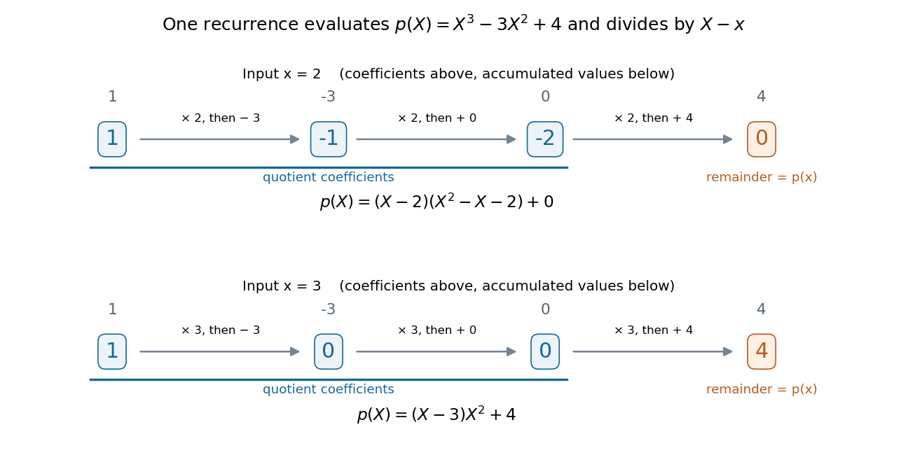
The same nested arithmetic evaluates a polynomial and produces the coefficients for division by a linear factor
. Details. 
The intermediate values do more than evaluate. They are the coefficients of the polynomial quotient in polynomial division by , with the final value as the polynomial remainder. At , the first three values give , soAt , they give , so . This links an efficient numerical calculation with the exact factor theorem.
William George Horner's 1819 paper concerns solving numerical equations by successive approximation. The Royal Society archive records the manuscript and its reading on 1 July 1819; it provides a historical reference for the method's name. [ref]
// Target: geometry-and-topology.bigb