Singular value decomposition

Singular Value Decomposition (SVD) is a mathematical technique in linear algebra used to factorize a matrix into three other matrices. It is particularly useful for analyzing and reducing the dimensionality of data, solving linear equations, and performing principal component analysis.

Ervand Kogbetliantz refers to a prominent figure known for his contributions to the fields of mathematics, engineering, and possibly the art of persuasion or communication. He is recognized for his work during the mid-20th century and has a legacy in academic and intellectual circles. However, it is important to verify details regarding specific contributions, publications, or particular areas of expertise associated with Kogbetliantz, as the name may not be widely recognized outside specialized fields.

Gene H. Golub

 0  0

Gene H. Golub was a prominent American mathematician known for his contributions to numerical analysis and linear algebra. He was born on January 28, 1932, and passed away on November 16, 2021. Golub is particularly recognized for his work on algorithms for matrix computations, including the singular value decomposition (SVD) and various methods for solving large-scale linear systems. He was a professor emeritus at Stanford University and made significant contributions to various fields of applied mathematics.

Normal mode

 1  0

"Normal mode" can refer to different concepts depending on the context in which it is used. Here are a few interpretations: 1. **Physics and Engineering**: In this context, "normal mode" refers to a specific type of oscillation in a system where all parts of the system move in a coordinated way. For example, in mechanical systems, normal modes correspond to the natural frequencies of vibration.

Singular value

 1  0

Singular values are a set of values that arise from the singular value decomposition (SVD) of a matrix. The SVD is a fundamental technique in linear algebra and statistics that is used to factorize a matrix into three other matrices.

Two-dimensional singular-value decomposition

 0  0

Two-dimensional Singular Value Decomposition (2D SVD) is a concept employed mainly in image processing and data analysis, where data is represented as a two-dimensional matrix (e.g., an image represented by pixel intensity values). It is an extension of the traditional singular value decomposition (SVD), which is typically applied to one-dimensional matrices (vectors) or higher-dimensional tensors.

 Ancestors (5)

 View article source

 Discussion (0)

New discussion

There are no discussions about this article yet.

 Articles by others on the same topic (1)

Singular value decomposition by

Codex  0 Created 2026-09-24 Updated 2026-10-14

 View more

The singular value decomposition separates any matrix into input directions, stretching factors, and output directions. Every

m \times n

complex matrix admits

A = U Σ V^{*}, U \in C^{m \times m}, Σ \in R^{m \times n}, V \in C^{n \times n} .

(1)

Here

U, V

are unitary matrices,

V^{*} = V^{†}

is the conjugate transpose, and

Σ

is a rectangular diagonal matrix. Its

p = min (m, n)

diagonal entries are the singular values, ordered

σ_{1} \geq \dots \geq σ_{p} \geq 0

. We use the conventional letters:

V

contains the right singular vectors

v_{j}

, while

U

contains the left singular vectors

u_{j}

. Writing

A = V Σ U^{†}

instead merely swaps these two matrix names; it requires swapping their roles consistently. For real matrices, choose orthogonal matrices and replace the conjugate transpose with the transpose.^[ref]

Reading from right to left,

V^{*}

expresses the input in an orthonormal basis,

Σ

stretches or annihilates those coordinates, and

U

assembles the output in another orthonormal basis. Unlike matrix similarity, the input and output bases can differ, and even have different sizes. A

3 \times 2

matrix has full factors of sizes

3 \times 3

3 \times 2

, and

2 \times 2

. If its matrix rank is

2

, one can retain only the active columns, giving sizes

3 \times 2

2 \times 2

, and

2 \times 2

for

U_{r}, Σ_{r}, V_{r}^{*}

; the full

U

additionally describes an unused output direction.

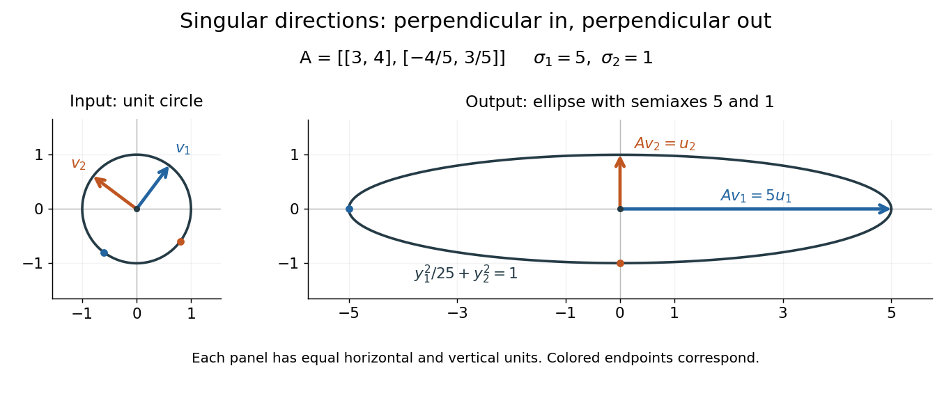
For a fully computed nonsymmetric example, take

A = (3 - 4/5 4 3/5), U = I, Σ = (5001), V = \frac{1}{5} (34 - 4 3) .

(2)

Multiplication gives

U Σ V^{T} = A

. The right singular vectors are

v_{1} = (3, 4)^{T} /5

and

v_{2} = (- 4, 3)^{T} /5

; their images are

A v_{1} = (5, 0)^{T}

and

A v_{2} = (0, 1)^{T}

. Thus, parametrizing the unit circle by

x = v_{1} cos t + v_{2} sin t

gives

A x = (5 cos t, sin t)^{T}

. Its image is the ellipse

y_{1}^{2} /25 + y_{2}^{2} = 1

. The two singular values are its semiaxis lengths, and the left singular vectors point along its axes. The singular value decomposition finds precisely the perpendicular input directions whose images stay perpendicular.

Figure 1.
The unit circle becomes an ellipse: $A v_{1} = 5 u_{1}$ and $A v_{2} = u_{2}$
. **Details**.

For compression, write the matrix as a sum of outer products and retain the largest terms:

A = \sum_{j = 1}^{r} σ_{j} u_{j} v_{j}^{*}, A_{k} = \sum_{j = 1}^{k} σ_{j} u_{j} v_{j}^{*}, ∥ A - A_{k} ∥_{F}^{2} = \sum_{j = k + 1}^{r} σ_{j}^{2},

(3)

where

r

is the matrix rank. Among all matrices of matrix rank at most

k

A_{k}

minimizes the Frobenius norm error; this is the Eckart-Young-Mirsky theorem. The operator norm error is

σ_{k + 1}

for

k < r

. These statements concern specified norms, rather than guaranteeing that discarded details are visually or scientifically unimportant.^[ref]

Consider an

8 \times 10

brightness matrix

B = p q^{T} + a b^{T} /2

, with

p = (1, 2, 3, 4, 4, 3, 2, 1)^{T}, q = (1, 2, 3, 4, 5, 5, 4, 3, 2, 1)^{T},

(4)

and

a_{i} = (- 1)^{i - 1}

b_{j} = (- 1)^{j - 1}

. The broad bright patch

p q^{T}

and alternating checkerboard

a b^{T} /2

have orthogonal row and column directions:

p^{T} a = q^{T} b = 0

. Their singular values are

60 \cdot 110 = 6600

and

8 \cdot 10 /2 = 20

. This low-rank approximation keeps the first outer product, giving

B_{1} = p q^{T}

, with Frobenius norm error

20 \approx 4.472

and relative error

20/6620 \approx 5.50%

. For example,

B_{11} = 1.5

becomes

1

, and

B_{12} = 1.5

becomes

2

: every entry changes by

0.5

in magnitude. The discarded pattern is small but entirely lost.

Figure 2.
An $8 \times 10$ matrix, its rank-one approximation, and the discarded checkerboard
. **Details**.

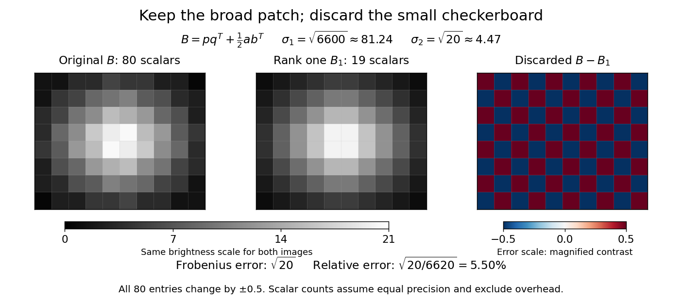
For this illustrative image compression, storing one normalized left singular vector, one normalized right singular vector, and one singular value requires

8 + 10 + 1 = 19

scalars instead of

80

. This counts scalars at equal precision, before storage overhead. In general,

k (m + n + 1)

scalars beat

mn

only for sufficiently small

k

, and small error requires a small discarded sum of squared singular values. The usefulness comes from measuring the tradeoff before throwing information away.^[ref]

 Read the full article

  See all articles in the same topic Create my own version

 Discussion (0)  Subscribe (1)

 Discussion (0)