 Euler method

The Euler method approximates an initial value problem $y^{\prime }=f(t,y)$, $y(t_0)=y_0$, by evaluating the derivative at the current point and moving along that tangent line for a time $h$. With $t_n=t_0+nh$, its displayed update needs one evaluation of $f$ per step. This simple rule turns local slope information into a whole approximate trajectory. MIT's course notes derive it by dropping the second-order Taylor remainder.^[ref]

Take $y^{\prime }=-2y$, $y(0)=1$, whose exact solution is the exponential function $y(t)=e^{-2t}$. The Euler method givesAt $h=0.2$, the first values are $1,0.6,0.36,0.216$. At $t=1$, five steps give $0.6^5=0.07776$, compared with $e^{-2}\approx 0.135335$. The result decays but is too small: absolute stability alone does not ensure accuracy. At $h=1.2$, the first values are $1,-1.4,1.96,-2.744$, and at $t=6$ five steps give $-5.37824$, while the exact solution is about $0.00000614421$.

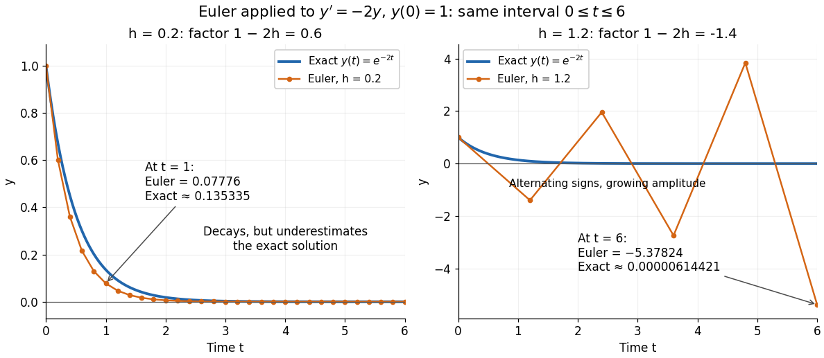
For the Dahlquist test equation $y^{\prime }=\lambda y$, the Euler method has stability function $R(z)=1+z$ with $z=h\lambda$. Its absolute stability region is $|1+z|\le 1$, the closed disk centred at $-1$ with radius one. For the present real decay problem and $h>0$, bounded numerical values require $0<h\le 1$; strict decay requires $0<h<1$. At $h=1$ the values alternate $1,-1,1,\dots$ without decay. These conditions follow directly from the amplification factor $1-2h$, matching MIT's criterion for $y^{\prime }=-ay$.^[ref]

The Euler method is first order: with bounded second derivative and suitable Lipschitz continuity, its global error is $O(h)$ on a fixed interval. In this example the logarithm gives $\log (1-2h)=-2h-2h^2+O(h^3)$ for small positive $h$. At $t=nh$, this means $y_n=e^{-2t}(1-2th+O(h^2))$. It explains both the downward bias and why halving the step roughly halves the error once $h$ is sufficiently small.