An initial value problem combines an ordinary differential equation with an initial condition, for example and . The task is to find a solution of a differential equation on an interval containing which has that starting value. For a continuous linear differential equation , every prescribed finite vector determines a unique solution on the coefficient interval. A boundary value problem can instead prescribe values at distinct endpoints.
For the cooling initial value problem , , where and are constant, the unique solution isTake degrees Celsius, degrees Celsius, , and per minute. Then degrees Celsius. Reaching degrees Celsius requires , so minutes. The time constant minutes reduces the excess temperature by a factor ; it does not reduce the absolute temperature by that factor.
Uniqueness needs assumptions. If is a continuous function on an open neighborhood of and satisfies a local Lipschitz condition in , uniformly in , the Picard-Lindelöf theorem gives a unique local solution. Concretely, a finite bounds in a sufficiently small rectangle. Cooling satisfies this with . Local existence does not promise existence for all future time: , , has on and finite-time blowup at .
Continuity alone is insufficient for uniqueness. Consider the dimensionless initial value problem involving a square root and an absolute value:Besides , each delay gives a solution for :At , delays give , despite identical starting data. These are valid solutions of a differential equation: for , both one-sided derivatives at the join are zero; for , the right derivative at the starting time is zero. After the join, because . Squaring alone would also suggest a parabola before the join, but its negative derivative there would violate the equation. Since , a forward solution starting from zero stays nonnegative.
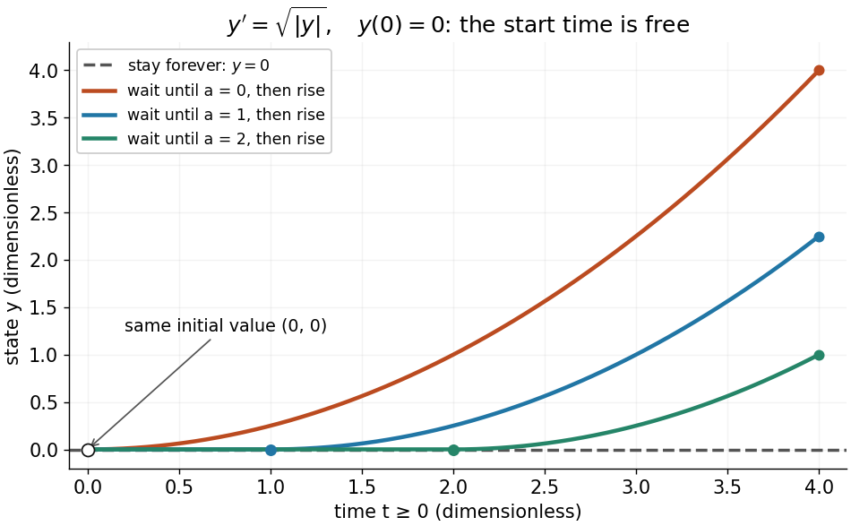
One initial value permits infinitely many delayed-start solutions without a Lipschitz condition
. Details. 
The right-hand side is a continuous function but fails the Lipschitz condition at zero: for , is unbounded. Thus the Peano existence theorem still supplies local existence, while the Picard-Lindelöf theorem does not supply uniqueness. Related waiting-time examples and a sufficient uniqueness condition appear in MIT 18.034, Lecture 2: Fundamental Principles.
A brief proof outline explains the mechanism: rewrite the initial value problem as the integral equation . On a short enough interval, the Lipschitz condition makes the right-hand side a contraction mapping on a closed set of continuous functions near . The contraction mapping theorem gives a unique fixed point; the fundamental theorem of calculus turns it back into a solution.
The displayed implicit ordinary differential equation has a singular initial point at the origin. On a nonconstant regular branch, treating as a function of gives . The integrating factor yields the first integral of an ordinary differential equationOne can verify this identity without dividing by : its derivative along a solution is .
The initial point forces , so . Near the origin this gives the two differentiable solutions and , with initial slopes zero and one. A division by would lose the first solution. A piecewise switch between the two at zero would fail differentiability because their one-sided slopes differ.
There is no conflict with the Picard-Lindelöf theorem: solving explicitly for requires division by , which vanishes at the initial point. A regular implicit equation or a local uniqueness theorem must be checked before claiming a unique solution through a singular point.
An L2 initial condition specifies a square-integrable initial function up to equality almost everywhere. It need not have pointwise nodal values or classical derivatives. L2-compatible initialization of grid data uses bounded averaging or projection, and evolution estimates use the relevant L2 norm.
Articles by others on the same topic
There are currently no matching articles.