 Laminar flow

Laminar flow is a regime of fluid flow in which the motion remains organized, with neighboring fluid parcels following smooth, coherent paths rather than the irregular interacting fluctuations characteristic of turbulence. In a straight pipe, the simplest example consists of coaxial layers sliding past one another. This describes the character of the motion, not a requirement that every parcel have the same velocity. Nor does it require steady flow: a smooth profile can evolve in time as viscosity transmits motion from a newly moving wall into a resting fluid. The unsteady wall-driven solution provides an explicit example. ^[ref]

The Reynolds pipe-and-dye experiment makes this distinction visible. A thin injected dye band can remain coherent in laminar flow, whereas irregular motion can fold it and carry dye across the pipe. However, molecular diffusion can spread dye even in laminar flow, and an inlet disturbance can move a coherent band without producing turbulence. A dye band is a streakline, not a measurement of the entire velocity field; in steady flow an ideal passive tracer's streakline coincides with a streamline. Reynolds explicitly distinguished a wandering band from one broken into eddies. ^[ref]

For a circular pipe of internal diameter $D$, define the mean axial velocity $U$ using the volumetric flow rate $Q$ and cross-sectional area $A$:Here $\rho$ is mass density, $\mu$ is dynamic viscosity and $\nu =\mu /\rho$ is kinematic viscosity. This particular Reynolds number uses the diameter and mean velocity, not the radius or centreline velocity. Small Reynolds number generally favors laminar flow, but a single universal critical Reynolds number does not distinguish it from turbulence in all geometries and experiments. Even in a given pipe, inlet conditions and the magnitude of disturbances affect the observed onset. Reynolds demonstrated this dependence by deliberately inserting a wire coil. ^[ref]

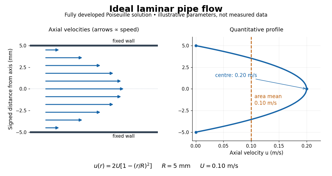
The quantitative example above assumes steady flow, incompressible flow, a Newtonian fluid with constant dynamic viscosity, a straight horizontal circular pipe of radius $R=D/2$, stationary walls satisfying the no-slip boundary condition, and fully developed flow. The last assumption means that the axial velocity profile no longer changes downstream. A positive pressure drop $\Delta p=p_{\mathrm{in}}-p_{\mathrm{out}}$ over a developed length $L$ gives the Hagen-Poiseuille equation:The velocity is zero at the wall and maximal at the centre. Averaging over the circular area, whose annuli have area $2\pi rdr$, gives $U=u(0)/2$; averaging along one diameter would give a different answer. These assumptions produce a parabola, rather than every laminar flow having a parabolic profile. ^[ref]

As a stipulated calculation, take $D=0.010\mathrm{m}$, $U=0.10\mathrm{m}{\mathrm{s}}^{-1}$, $\rho =1000\mathrm{kg}{\mathrm{m}}^{-3}$, $\mu =0.0010\mathrm{Pa}\mathrm{s}$ and $L=1.0\mathrm{m}$, and assume the developed laminar flow above. Then $\nu =10^{-6}{\mathrm{m}}^2{\mathrm{s}}^{-1}$, ${\mathrm{Re}}_D=1000$, $u(0)=0.20\mathrm{m}{\mathrm{s}}^{-1}$, $Q=7.85\times 10^{-6}{\mathrm{m}}^3{\mathrm{s}}^{-1}$ (about $0.471\mathrm{L}\mathrm{mi}{\mathrm{n}}^{-1}$), and $\Delta p=32\mu LU/D^2=32\mathrm{Pa}$. These are predictions from chosen parameters, not measurements or a claim that ${\mathrm{Re}}_D=1000$ guarantees laminar flow in every apparatus.

The beauty of this example is that a spatially varying velocity field still gives an exact relation between two accessible measurements, pressure drop and volumetric flow rate. It predicts the hydraulic resistance $\Delta p/Q=8\mu L/(\pi R^4)$. Doubling the radius therefore multiplies $Q$ by sixteen at fixed pressure drop, length and dynamic viscosity, provided the model remains applicable. This makes the laminar flow model useful for sizing narrow tubes or determining dynamic viscosity. It also explains why a persistent narrow dye band can be informative without implying that the fluid is moving as a uniform plug.