Maser oscillation threshold
ID: maser-oscillation-threshold

The following original model isolates amplification by inverted electric dipoles. Let be the excess number in the upper member of one equally degenerate resonant pair. Let be a slowly varying cavity amplitude with photon number , and let describe the collective molecular dipole component in the amplifying phase convention. On exact resonance, stipulate the linear equationsThe dipole relaxation rate is , and is a single-molecule coupling in the chosen mode normalization. Here is an electric dipole moment matrix element, is the field's zero-point amplitude, and . Field overlap and dipole orientation enter this coupling. The characteristic polynomial for growth rate isFor , one root becomes positive precisely when . If dipole relaxation is fast enough to eliminate , then andThus positive population inversion alone is insufficient: the gain rate must exceed the passive decay rate. This reduction describes the onset near resonance; it does not predict output phase noise, actual transit dynamics or an exact historical threshold. Nikolay Basov and Aleksandr Prokhorov's molecular-generator theory likewise treats self-excitation as competition between molecular gain and resonator-plus-load losses.[ref]
Theory of the Molecular Generator and Molecular Power Amplifier by Nicolay Gennadiyevich Basov and Aleksandr Mikhailovich Prokhorov. p. 426, Introduction; pp. 427–428, dipole response and self-excitation
To include replenishment, suppose upper-state molecules enter at rate and both levels leave with residence rate . A deliberately simple ordinary differential equation model isOne downward transition removes two units of the difference , so . Below onset the unsaturated inversion is , givingFor fixed mode volume , the equivalent number density condition is . Raising selected beam intensity raises gain; increasing quality factor lowers the loss rate at fixed frequency. These statements hold with , residence time and mode overlap fixed.
Above onset, the nonzero steady state hasThe inversion is clamped while excess supply supports output. A finite initial seed is understood: the noiseless equations leave exactly unchanged even above onset. Actual startup has spontaneous emission and field fluctuations.
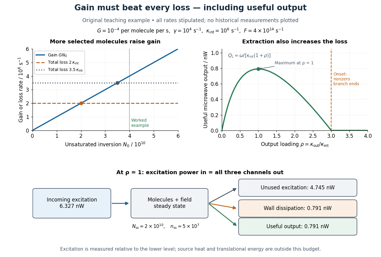
Maser oscillation threshold, output loading and the maser microwave energy budget
. Original illustrative model, not historical measurements. Left: gain rises with selected beam supply, crossing two chosen total loss rates. Right: with fixed supply, output initially grows with output coupling, then falls to zero when that coupling makes the total loss too large. The lower panel accounts for incoming excitation, unused excitation leaving in the beam, wall dissipation and useful output for the worked example. Details.
New to topics? Read the docs here!