
A morphogen gradient is a spatially varying concentration profile of a morphogen. The profile specifies the local amount; its mathematical gradient, in one dimension, specifies how rapidly that amount changes with position. In the simplest positional interpretation, a biological cell responds to its local concentration, without having to measure the gradient across itself. Production, transport and removal together determine a morphogen gradient.
For a worked example, take a stationary one-dimensional tissue occupying , constant diffusion coefficient , and uniform first-order reaction removal at rate . At steady state, this specialization of the morphogen reaction-diffusion equation gives the ordinary differential equation and boundary conditionsHere has units of length squared per time, has units of inverse time, and is a prescribed source concentration. The Dirichlet boundary condition fixes the concentration at . It does not prescribe a source flux; any required flux follows from the solution. These assumptions define a toy morphogen gradient, not a universal account of transport during biological development.
Define the diffusion length . Substitution into the ordinary differential equation shows that its general solution is . The vanishing boundary condition at infinity forces , and the source Dirichlet boundary condition forces . HenceOver every additional diffusion length, the concentration falls by the same factor . Faster diffusion increases ; faster removal decreases . This makes the diffusion length a useful bridge between microscopic transport and the spatial reach of a morphogen gradient.
Choose arbitrary concentration units and , where . Then : at , and , the concentrations are , approximately and approximately . The following diagram combines this morphogen gradient with the idealized responses calculated under morphogen response threshold.
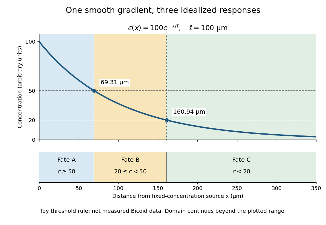
A toy morphogen gradient and three idealized developmental bands
. The steady state profile uses arbitrary concentration units and diffusion length . Morphogen response thresholds at and place the boundaries at approximately and . The lower strip shows assigned fates A, B and C, not measured tissues. The plotted domain ends at ; the mathematical domain continues to infinity. Details.
New to topics? Read the docs here!