Negative binomial distribution
ID: negative-binomial-distribution

The negative binomial distribution counts failures before a target number of successes in successive independent Bernoulli trials with constant success probability . In this stopping model, is a positive integer and . On the failures-before-the-th-success convention, the random variable takes values ; for , its probability mass function isThe binomial coefficient counts possible arrangements before the final success, as explained by the negative binomial stopping argument. At , every trial succeeds: with probability one, so its expected value and variance are both zero. This handles the endpoint without needing to interpret . At , the target is never reached and there is no proper finite waiting-count law.
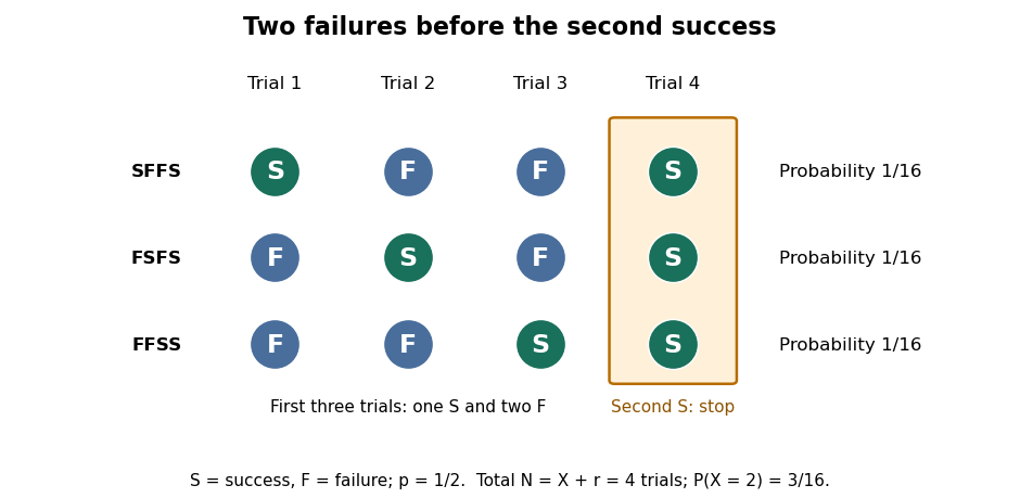
For a worked example, toss a fair coin until the second head, calling heads and tails . Thus and . Exactly two failures means that the second success is on trial four. The complete stopped sequences are , and ; each has probability , giving . The first three masses areBoth and are modes, each with mass : there is no unique mode here. Later masses decrease, since for .
The expected value and variance of the failures count areIf instead counts all trials, including the successes, then andFor the fair-coin example, , , and . Shifting the count changes its expected value but preserves its variance. When , has the failures-count geometric distribution, while has the all-trials geometric distribution. The two conventions and the moments are treated in Kyle Siegrist, The Negative Binomial Distribution, Random Services.
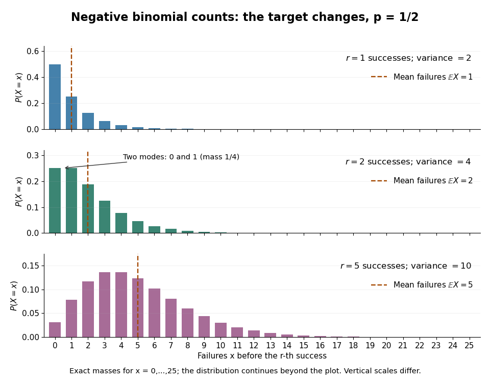
Negative binomial failure counts for success probability 1/2 and targets of one, two and five successes
. Details. The negative binomial distribution is useful when a procedure runs until it collects a target number of successes: for example, obtaining usable samples from independent attempts with a stable acceptance probability. A binomial distribution instead counts successes in a fixed number of trials. The attractive connection is that these two experimental questions can be answered from the same trial sequence, using the negative binomial stopping argument. For the failures count and , the positive mean satisfies , so the law allows overdispersion relative to a Poisson distribution. At , both quantities vanish and the inequality is not strict. The separate Poisson-gamma mixture explains another way this count law arises; its noninteger shape parameters do not represent a literal target number of successes.



The Negative Binomial distribution is a discrete probability distribution that models the number of trials needed to achieve a fixed number of successful outcomes (often referred to as "successes"). It is commonly used in scenarios where we are interested in the number of failures that occur before a certain number of successes is achieved. ### Key Characteristics: 1. **Parameters**: The Negative Binomial distribution is defined by two parameters: - \( r \): the number of successes (a positive integer).
New to topics? Read the docs here!