Noise covariance between windowed Fourier bins
ID: noise-covariance-between-windowed-fourier-bins

Noise covariance between windowed Fourier bins describes the statistical dependence created when several spectral estimates use the same noisy record. A window changes not only each estimate’s equivalent noise bandwidth, but also the overlap of their frequency responses. Uncorrelated time samples therefore need not produce uncorrelated spectral bins after tapering.
Let independent zero-mean sample errors satisfy . Use real coefficients , nonzero sum , and coherent-amplitude-normalized estimates on the original -point grid,Expanding their complex covariance and removing the vanishing cross terms givesThus the covariance is the Fourier transform of the squared window, evaluated at the bin difference. Its diagonal agrees with the equivalent noise bandwidth variance formula. SciPy’s spectrum/density scaling likewise uses the coefficient-square sum separately from the squared coherent sum.[ref]
For a rectangular window, the exponential orthogonality sum gives on this unpadded grid. This is a statement about covariance; independence additionally follows for an appropriate Gaussian noise model, not for every possible input distribution.
For the periodic Hann window, with ,Its original-grid covariance has only five nonzero cyclic diagonals:with bin indices modulo . Normalizing by the common diagonal gives adjacent-bin covariance ratio and second-neighbor ratio . The negative sign follows from this window’s placement in the record; changing the time placement can change covariance phases without changing their magnitudes. The periodic and symmetric coefficient conventions must not be interchanged in this finite calculation.[ref]
SciPy 1.16.2 documentation. scipy.signal.windows.hann, sym parameter and defining raised-cosine coefficients
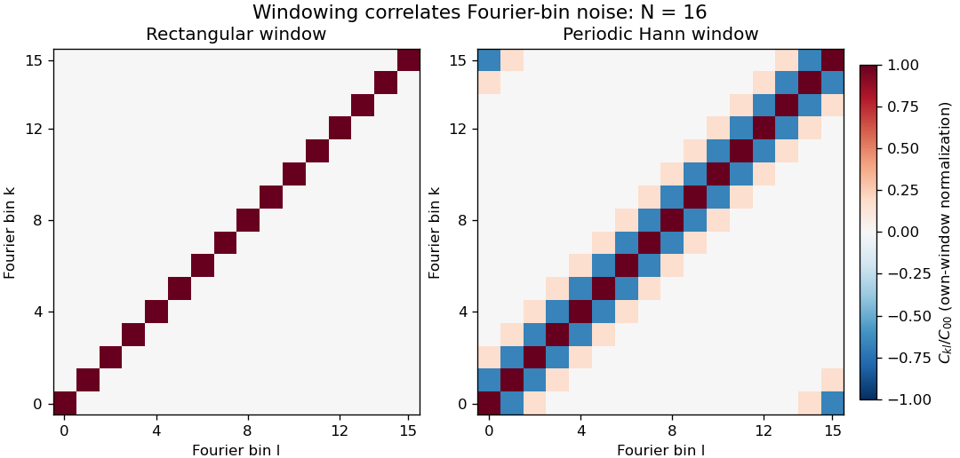
Noise covariance between windowed Fourier bins for rectangular and periodic Hann windows
. Exact original N=16 grid covariance matrices for independent equal-variance sample errors. Each matrix is divided by its own diagonal variance, so the plot compares correlation structure rather than absolute noise level. The corner bands arise from cyclic bin indexing. No sampled experimental data or random simulation is used. Details.
Correlation of neighboring periodogram powers is different from the sign of this complex covariance. Suppose each input sample has independent Gaussian real and imaginary parts, each of variance , with all components independent across time. The nonconjugated second moments vanish. Gaussian fourth-moment pairing, as in Isserlis's theorem, then givesConsequently neighboring Hann-bin powers are positively correlated despite the negative covariance of their complex amplitudes. If , their individual power variances are , and the variance of their arithmetic mean isTreating them as independent would incorrectly give . For real Gaussian input, a further term enters the power covariance; the pseudo-covariance of a complex random variable and conjugate-frequency symmetry therefore need attention near paired bins and the real-valued endpoint bins.
Zero padding creates more closely spaced evaluations of the same record, not more independent noise realizations. Even a rectangular record generally has correlated estimates on that denser grid. Detrending, colored input noise and overlapping records change the covariance calculation too. SciPy exposes detrending and FFT-length choices explicitly; its default constant detrending must be disabled when testing the unmodified independent-sample model above.[ref]
A proposed numerical check generates many independent records with the stated noise distribution, computes the estimates with fixed coefficients, and compares empirical complex covariance and power covariance separately with the formulas. A physical noise test additionally needs a characterized acquisition bandwidth and an assessment of time-sample correlation. Averaging several correlated spectral values does not supply the same precision gain as averaging independent records.
New to topics? Read the docs here!