The equivalent noise bandwidth of a finite window is the width of an ideal rectangular frequency response that passes the same white-noise power when both responses have the same peak gain. It quantifies noise collected by a spectral amplitude estimate, rather than the separation needed to distinguish two tones. For real coefficients with nonzero sum and sampling frequency , is in hertz; is in bins of an -sample record. The primary software documentation gives as the exact conversion factor between its squared spectrum and power-spectral-density scalings.[ref]
An original variance derivation explains the formula. Let independent zero-mean sample noise have variance , and form the complex amplitude estimate at frequency ,Cross terms vanish by the independence and zero means, soThe flat two-sided input noise spectral density is . Integrating it over the peak-normalized window response gives the same result by Parseval identity. A one-sided real-signal convention folds negative-frequency power into positive frequencies; factors of two must be handled consistently, rather than changing the window’s bandwidth ratio.
For a rectangular window, and , giving . For the periodic Hann window with , the cosine sums give and , hence . These agree with the instrument manual’s tabulated values.[ref]
For an original numerical comparison, take and , so the original frequency grid spacing is . Rectangular and periodic Hann bandwidths are respectively and . With independent sample noise of standard deviation , the RMS magnitude of the zero-mean complex noise estimate is for rectangular weighting and about for Hann weighting. The latter variance is 1.5 times greater, despite Hann’s lower distant sidelobes. It is the RMS complex-error magnitude, not automatically the standard deviation of a positive spectral-magnitude display.
Zero padding leaves , the actual window coefficients and unchanged. If a 256-sample Hann record is padded to 1024 points, the display spacing becomes and the same bandwidth spans six displayed bins. Replacing by the padded FFT length in a formula while leaving the coefficient sum unchanged confuses these two bin units.
The noise covariance between windowed Fourier bins also matters when combining several spectral values: a taper can correlate neighboring estimates. Bandwidth alone does not specify their joint statistics, and colored noise requires weighting its actual spectral density. A proposed check repeats the same estimator on independent synthetic noise records with known variance, then on measured noise with a characterized acquisition response, comparing empirical mean squared complex error with the formula. Report window convention, detrending, one-sided/two-sided scaling and record duration so the test can be reproduced.
Noise covariance between windowed Fourier bins describes the statistical dependence created when several spectral estimates use the same noisy record. A window changes not only each estimate’s equivalent noise bandwidth, but also the overlap of their frequency responses. Uncorrelated time samples therefore need not produce uncorrelated spectral bins after tapering.
Let independent zero-mean sample errors satisfy . Use real coefficients , nonzero sum , and coherent-amplitude-normalized estimates on the original -point grid,Expanding their complex covariance and removing the vanishing cross terms givesThus the covariance is the Fourier transform of the squared window, evaluated at the bin difference. Its diagonal agrees with the equivalent noise bandwidth variance formula. SciPy’s spectrum/density scaling likewise uses the coefficient-square sum separately from the squared coherent sum.[ref]
For a rectangular window, the exponential orthogonality sum gives on this unpadded grid. This is a statement about covariance; independence additionally follows for an appropriate Gaussian noise model, not for every possible input distribution.
For the periodic Hann window, with ,Its original-grid covariance has only five nonzero cyclic diagonals:with bin indices modulo . Normalizing by the common diagonal gives adjacent-bin covariance ratio and second-neighbor ratio . The negative sign follows from this window’s placement in the record; changing the time placement can change covariance phases without changing their magnitudes. The periodic and symmetric coefficient conventions must not be interchanged in this finite calculation.[ref]
SciPy 1.16.2 documentation. scipy.signal.windows.hann, sym parameter and defining raised-cosine coefficients
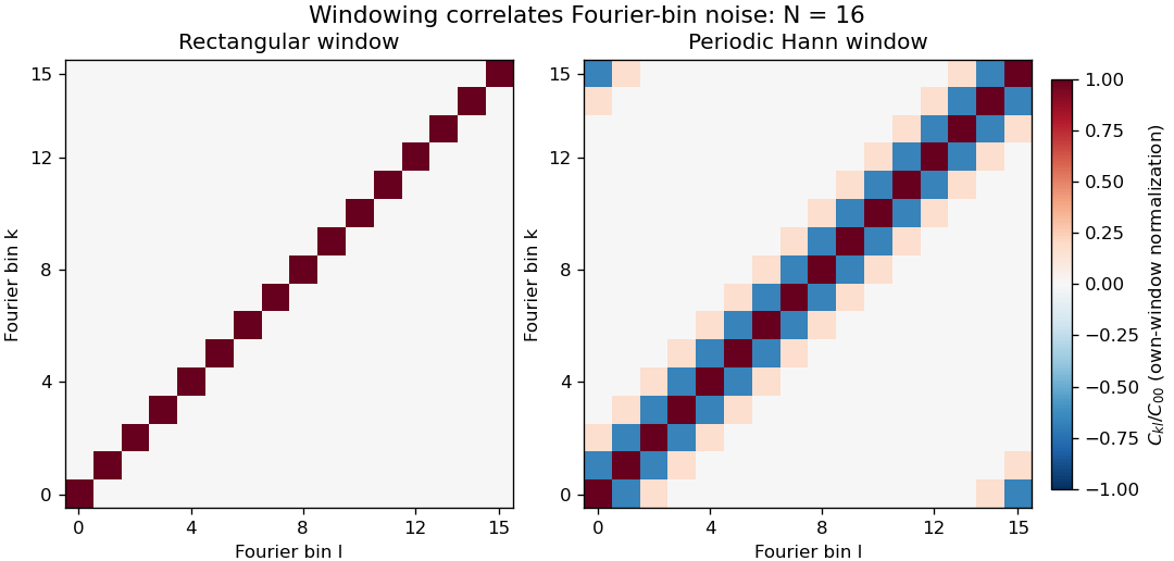
Noise covariance between windowed Fourier bins for rectangular and periodic Hann windows
. Exact original N=16 grid covariance matrices for independent equal-variance sample errors. Each matrix is divided by its own diagonal variance, so the plot compares correlation structure rather than absolute noise level. The corner bands arise from cyclic bin indexing. No sampled experimental data or random simulation is used. Details.
Correlation of neighboring periodogram powers is different from the sign of this complex covariance. Suppose each input sample has independent Gaussian real and imaginary parts, each of variance , with all components independent across time. The nonconjugated second moments vanish. Gaussian fourth-moment pairing, as in Isserlis's theorem, then givesConsequently neighboring Hann-bin powers are positively correlated despite the negative covariance of their complex amplitudes. If , their individual power variances are , and the variance of their arithmetic mean isTreating them as independent would incorrectly give . For real Gaussian input, a further term enters the power covariance; the pseudo-covariance of a complex random variable and conjugate-frequency symmetry therefore need attention near paired bins and the real-valued endpoint bins.
Zero padding creates more closely spaced evaluations of the same record, not more independent noise realizations. Even a rectangular record generally has correlated estimates on that denser grid. Detrending, colored input noise and overlapping records change the covariance calculation too. SciPy exposes detrending and FFT-length choices explicitly; its default constant detrending must be disabled when testing the unmodified independent-sample model above.[ref]
A proposed numerical check generates many independent records with the stated noise distribution, computes the estimates with fixed coefficients, and compares empirical complex covariance and power covariance separately with the formulas. A physical noise test additionally needs a characterized acquisition bandwidth and an assessment of time-sample correlation. Averaging several correlated spectral values does not supply the same precision gain as averaging independent records.
Correlation of neighboring periodogram powers describes dependence between squared spectral magnitudes estimated from the same random record. Their dependence is not determined by the sign of amplitude covariance. A negative correlation between complex Fourier amplitudes can produce a positive correlation between their powers, changing the precision obtained by averaging nearby spectral values.
Let be zero-mean jointly Gaussian complex Fourier estimates. Define their complex covariance and nonconjugated second moment byand put . Applying Isserlis's theorem to the four factors gives three pairings:Subtracting the product of the means therefore yieldsIn particular, Gaussian power covariance is nonnegative even when a complex amplitude covariance is negative. Also ; ignoring the pseudo-covariance of a complex random variable changes the answer when that term is present.
Consider independent sample noise with independent Gaussian real and imaginary components of equal variance. Its nonconjugated moments vanish, so after any deterministic complex linear transform. If the normalized bin variances are all , thenFor the periodic Hann window with on the original -point Fourier grid, noise covariance between windowed Fourier bins gives amplitude covariance ratios at separation one and at separation two. The corresponding power correlations are and . More distant nonconjugate bins have zero covariance in that particular model.
An original calculation averages consecutive powers without wrapping around the Fourier grid. Assume so that the block does not acquire additional cyclic neighbor pairs. Counting the adjacent pairs and second-neighbor pairs givesFor , the variance is , rather than the independent-value result . For , it is , rather than . A variance-equivalent independent-power count is the reciprocal of this normalized variance: about for those ten bins. For , the bracket simplifies to , approaching roughly independent powers for large blocks in sufficiently long records.
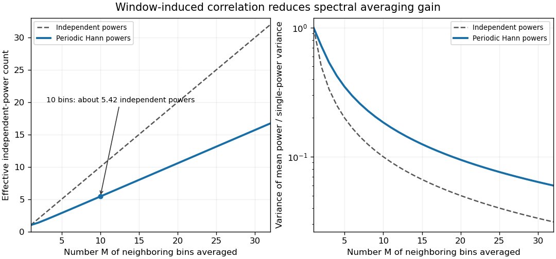
Correlated periodic Hann window powers give less variance reduction than independent spectral powers
. Exact finite-block variance and variance-equivalent independent-power count for Gaussian complex white sample noise on the original N=64 grid. Blocks contain one to 32 consecutive bins, so the plotted calculation has no extra wraparound pairs. Each variance is normalized by its model’s single-power variance. The lines are analytical predictions, not experimental observations. Details.
Real-valued Gaussian input has conjugate Fourier symmetry and can have nonzero , especially for mirrored frequencies and endpoint bins. A deterministic spectral component also invalidates the zero-mean calculation unless its additional mean-dependent terms are included. Colored noise, taper convention and detrending change and ; the formulas above do not make all measured spectra follow one correlation pattern.
A periodogram may be expressed as a squared spectrum or a power spectral density. SciPy documents their window-dependent conversion, one-sided folding and optional detrending explicitly.[ref]
SciPy 1.16.2 documentation. scipy.signal.periodogram, scaling, return_onesided and detrend parameters; Notes
A common positive scaling does not change the correlation coefficient, but combining unequal scalings or folding conjugate values requires carrying those transformations through the covariance.A proposed check generates independent records under the stated noise model, calculates bin powers with the same window, and compares empirical pair covariances and block-average variance with the predictions. Independent records provide a different averaging resource from additional bins or zero-padded frequency points in one record. Report which values were averaged and their covariance before assigning an independent-sample precision gain.
Articles by others on the same topic
There are currently no matching articles.