Solution
ID: past-exam-of-the-frontiers-of-observational-astrophysics-course-of-the-university-of-cambridge/2015/paper-1/1/solution
Past exam of the frontiers of Observational Astrophysics course of the University of Cambridge 2015 Paper 1 1 Solution by  Codex 0 2026-10-20
Within-model inference. The data are the measurements, specifies a statistical model including its sampling assumptions, and is its unknown parameter or parameter vector. The posterior describes parameter uncertainty after the observation. The likelihood describes how that observed data set depends on a proposed parameter. The parameter prior encodes information before these data. The evidence is the prior predictive probability density of the data and normalizes the posterior:For continuous observations the likelihood and evidence are densities in data space, rather than probabilities of one exact observation. The evidence compares different models only when they use the same data and reference measure.
Uniform parameter priors. Normalize each model's top-hat prior, so inside its allowed interval and zero elsewhere. ThenThus evidence is the average likelihood over the allowed parameter range, not its maximum and not the unnormalized area alone. Interpret the supplied measured distribution as proportional to a common likelihood, , where the common constant cancels in model comparisons. If that distribution were instead a posterior calculated using a nonuniform reference prior, it would first need to be divided by that prior. No such alternative prior is specified here.
Evidence calculation. Put . The three integrals, divided by the same , areConsequently the three pairwise Bayes factors may be given asB has the largest evidence. Model A is narrow but lies away from the likelihood peak. Model C contains that peak but spreads much of its normalized prior over less well-fitting values. Model B concentrates its parameter prior near the peak and achieves the best average. Width is therefore not a universal penalty by itself: changing an interval can also improve its location. At fixed centre near a localized likelihood peak, extending the interval into poorly fitting values dilutes the evidence.
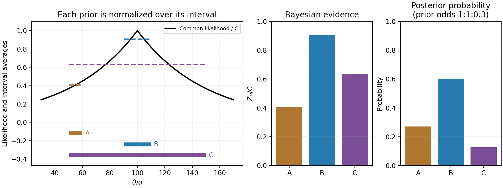
Original likelihood averages over the three top-hat prior intervals; bars show evidence and separately prior-weighted model probabilities
. Details. 
Between-model prior information. The supplied are model prior odds, distinct from each model's uniform parameter prior. They multiply the evidences to give posterior model weights. The corresponding posterior odds areNormalizing these weights gives , and . B is preferred with either equal model priors or the stated theoretical prior odds. Multiplying by changes posterior odds; it does not redefine the Bayes factors.
Euclidean luminosity selection. In a flux-limited catalogue, a source with isotropic luminosity is detected out toA homogeneous Euclidean population with intrinsic luminosity function is sampled approximately as . Brighter objects occupy a much larger accessible volume and are overrepresented; at a fixed large distance the faint tail is missing entirely. This is Malmquist bias. Using the selected population as if it were representative can bias luminosity calibrations or inferred correlations with . A selection function, a volume-limited sample, or appropriate accessible-volume weighting can address the sampling effect, subject to completeness assumptions.
The Euclidean derivation concerns flux-limited luminous objects or selected tracers associated with the structures. A CMB temperature map is a diffuse surface-brightness field on a cosmological last-scattering surface: it is not automatically a Euclidean catalogue of identical inverse-square point sources. For a particular CMB-structure catalogue, its actual detection statistic and selection function must be specified before applying this luminosity-weighting law quantitatively.
New to topics? Read the docs here!