Statistical model

A statistic is invariant if

A (g y) = A (y)

; it is maximal when it also separates different group orbits. Consequently every invariant procedure factors through the maximal invariant, subject to the usual measurability conditions on the orbit space. Standardizing a sample by an equivariant estimator of location and positive scale gives a maximal invariant for the positive affine group.

Ranks as a maximal invariant under increasing transformations

On samples of distinct real observations, the labeled rank vector is a maximal invariant for simultaneous strictly increasing bijections of the real line. Such transformations preserve every comparison. Conversely two samples with the same ranks can be matched by a piecewise linear increasing bijection through their corresponding ordered observations, with positive-slope tails. Under a common continuous probability distribution, every labeled ordering is equally likely by exchangeability, giving distribution-free rank tests. This argument does not assume that all continuous distributions lie in one orbit of real-line homeomorphisms.

Invariant tests factor through a maximal invariant

T

is a maximal invariant for a group action, an invariant test function is constant on each group orbit and therefore equals

b \circ T

for a function

b

on the orbit space. Conversely every such function is invariant. Appropriate quotient measurability is understood. If the action is transitive on a null family of probability distributions, invariance also gives the same null law of

T

under every member. Thus tests based on

T

eliminate that null nuisance variation.

Parametric statistical model ( ${P_{θ} : θ \in Θ \subseteq R^{d}}$ )

A statistical model indexed by a parameter vector of fixed finite dimension is parametric. Examples include a normal distribution with unknown mean and variance and a Poisson distribution with unknown mean. Its likelihood function is the joint sample density or mass function, regarded as a function of the parameter at the observed sample.

Location-scale family ( $f (y; μ, σ) = σ^{- 1} f_{0} ((y - μ) / σ)$ )

In a location-scale family,

Y = μ + σ Z

for a fixed base probability distribution of

Z

, with

μ \in R

and

σ > 0

. Location translates observations, and scale multiplies their deviations. For an independent sample with a base density and at least two observations, the normalized residual vector

(Y_{i} - \overset{ˉ}{Y}) / s

, where

s^{2} = n^{- 1} \sum_{i} (Y_{i} - \overset{ˉ}{Y})^{2}

, is an ancillary statistic. Indeed,

\overset{ˉ}{Y} = μ + σ \overset{ˉ}{Z}

and

s = σ s_{Z}

, making the residual vector a function of the base sample alone. This algebraic result needs no population moments.

Log-transformed location-scale model ( $lo g T = α + σW$ )

W

has probability density function

f (w; q)

and cumulative distribution function

F_{W} (w; q)

, then

T = exp (α + σW)

σ > 0

, has density

f ((lo g t - α) / σ; q) / (σ t)

and distribution function

F_{W} ((lo g t - α) / σ; q)

for

t > 0

. The factor

1/ (σ t)

follows from the change-of-variables formula for a probability density. Upper truncation at

M

divides the density by

F_{W} ((lo g M - α) / σ; q)

Conditional inference in a location-scale family ( $L_{μ, σ} (\overset{ˉ}{Y}, s ∣ A = a)$ )

For normalized residuals

A_{i} = (Y_{i} - \overset{ˉ}{Y}) / s

, Fisherian conditional inference uses the conditional distribution of

(\overset{ˉ}{Y}, s)

given the observed

A = a

. For almost every attainable ancillary value, the joint conditional density of

\overset{ˉ}{Y} = m

and

s = t > 0

is proportional to

t^{n - 2} σ^{- n} \prod_{i = 1}^{n} f_{0} (\frac{m + t a _{i} - μ}{σ}) .

The factor

t^{n - 2}

is the radial Jacobian on the

(n - 1)

-dimensional centered residual space. After setting

u = (m - μ) / σ

and

v = t / σ

, the conditional density is proportional to

v^{n - 2} \prod_{i} f_{0} (u + v a_{i})

, which is parameter-free. Conditioning on a continuous ancillary uses a regular conditional distribution, rather than division by the probability of a singleton ancillary value.

Regression model ( $f_{β} (y ∣ x)$ )

A regression model specifies features of the conditional distribution of a response given predictor covariates, often a conditional mean or a full parametric density. Linear regression specifies a linear conditional mean; logistic regression specifies a logit-linear conditional probability for a binary response. The conditional comparison represented by a coefficient depends on which covariates are included.

Interaction (statistics)

A statistical interaction means that the effect of one predictor depends on another on the chosen response scale. In a linear regression, an interaction term

β_{3} XZ

changes the slope in

X

β_{1} + β_{3} Z

. Whether interaction is present depends on the comparison scale; additive effects and multiplicative effects use different null contrasts. Comparing subgroup effects requires an interaction contrast, rather than contrasting their separate significance labels.

Interaction plot

An interaction plot displays response means against levels of one factor, with separate lines for levels of another and optional panels for further factors. In an additive linear regression, the difference between two lines is constant across the horizontal factor, so the population-mean lines are parallel. Changing line separations or crossings show a statistical interaction on that response scale. Sample means may be nonparallel through noise, so the plot describes the effect pattern rather than replacing a formal hypothesis test.

Interaction term

An interaction term lets the effect of one predictor depend on another. In

E [Y ∣ X, Z] = β_{0} + β_{1} X + β_{2} Z + β_{3} XZ,

the slope with respect to

X

β_{1} + β_{3} Z

Two-factor interaction

A two-factor interaction means that changing one factor has a different effect at different levels of another. For a two-level factorial design, its sign column is

x_{i} x_{j}

, and four times its coefficient is the corresponding difference of differences. It can be confounded with other factorial contrasts in a fractional factorial design.

Coupling constant (physics, $g$ )

A coefficient multiplying an interaction term controls its strength relative to the chosen field normalization. Its engineering dimension determines whether it is dimensionless, relevant or irrelevant. A renormalized coupling constant constant is specified at a renormalization scale; its change with that scale is described by the renormalization-group beta function.

Principle of marginality

A hierarchical statistical model that contains an interaction term retains its associated lower-order effects. For two categorical predictors this means keeping both main effects when keeping their interaction. A nonsignificant averaged main effect may coexist with large opposite effects in different groups. Dropping its lower-order term while retaining the interaction can make the model depend on arbitrary factor coding.

Statistical path ( $t \mapsto P_{t}, P_{0} = P$ )

A statistical path is a one-dimensional family of probability measures inside a statistical model, passing through a specified baseline

P

. A differentiability in quadratic mean condition gives its score function, the first-order direction of the family in square-root-density coordinates. The path must respect all restrictions of the statistical model, including normalization and any fixed moments.

Statistical tangent set ( $\dot{P}_{P}$ )

A statistical tangent set is the collection of score functions attained by a specified family of differentiable-in-quadratic-mean paths through

P

. The choice of paths is part of the definition. Its elements lie in the mean-zero L2 space, but the set need not already be a closed vector subspace.

Bounded density tilt ( $p_{t} = p (1 + t g), P g = 0$ )

For bounded measurable

g

with

P g = 0

, the formula

p_{t} = p (1 + t g)

defines a normalized positive probability density function for

∣ t ∣∥ g ∥_{\infty} < 1

. A uniform Taylor expansion of the square root proves differentiability in quadratic mean with score function

g

: the squared remainder is

O (t^{4} P g^{4})

. Such paths realize all bounded centered directions of an unrestricted density model.

Density of bounded centered scores ( $\overline{{g bounded : P g = 0}}^{L^{2} (P)} = L_{0}^{2} (P)$ )

For

h \in L_{0}^{2} (P)

, truncate

h

h_{m} = max (- m, min (h, m))

and subtract

P h_{m}

. Dominated convergence gives

h_{m} \to h

in L2 space, and the Cauchy-Schwarz inequality gives

P h_{m} \to 0

. Thus bounded centered directions are dense in the mean-zero L2 space. The measure defining the L2 norm is essential: density-weighted L2 space can contain functions outside the unweighted Lebesgue space.

Statistical tangent space ( $\overline{span} \dot{P}_{P}$ )

The statistical tangent space is the closed linear span in L2 space of a statistical tangent set. Taking this closure makes orthogonal projection available and ensures that a continuous derivative specified on attainable score functions extends to the whole space.

Differentiability in quadratic mean ( $∥ p_{t} - p - \frac{t}{2} g p ∥_{2} = o (∣ t ∣)$ )

A dominated statistical path is differentiable in quadratic mean at

P

if its square-root probability density function has an L2 space derivative

(1/2) g p

, with

g \in L^{2} (P)

. The score function is

g

. This formulation controls mass near zeros of

p

as well as the derivative on the support of

P

; a pointwise log-density derivative is insufficient by itself.

Quadratic-mean to L1 density derivative ( $∥ p_{t} - p - tp g ∥_{1} = o (∣ t ∣)$ )

Let

δ_{t} = p_{t} - p = (t /2) g p + r_{t}

, with

∥ r_{t} ∥_{2} = o (∣ t ∣)

. Since

p_{t} - p = 2 p δ_{t} + δ_{t}^{2}

, the Cauchy-Schwarz inequality gives

∥ p_{t} - p - tp g ∥_{1} \leq 2∥ r_{t} ∥_{2} + ∥ δ_{t} ∥_{2}^{2} = o (∣ t ∣)

. Thus differentiability in quadratic mean suffices to differentiate bounded density integrals, even when the density itself has no useful pointwise derivative.

Mean-zero score identity under quadratic-mean differentiability ( $P g = 0$ )

For a differentiable-in-quadratic-mean path, normalization gives

⟨(p_{t} - p) / t, p_{t} + p ⟩ = 0

. The two factors converge in L2 space to

g p /2

and

2 p

. Continuity of the inner product therefore gives

P g = 0

. This proves score function centering without differentiating the density integral.

Scale family ( $p (y ∣ σ) = σ^{- 1} f (y / σ)$ )

A scale family rescales a fixed distribution by a positive parameter. The standardized variable

Y / σ

has density

f

, independent of

σ

. This simplifies moments, simulations and the Jeffreys prior for a scale parameter.

Statistical parameter ( $θ \in Θ$ )

A statistical parameter indexes a family of probability distributions in a statistical model. It is fixed in a frequentist sampling model; a prior distribution makes it random for Bayesian statistics. Different statistical parameter values should produce different observable distributions when identifiability is claimed.

Nuisance parameter

A nuisance parameter is a statistical parameter required to specify the distribution of observations but not itself the target of inference. A profile likelihood maximizes over it; Bayesian model evidence integrates over it using a proper prior distribution. These operations differ and need not give the same inference. A baseline hazard in a Cox proportional-hazards model is an infinite-dimensional example.

Mixed log-likelihood derivative obstruction to parameter separation ( $\partial_{ψ} \partial_{λ} lo g f$ )

On a common positive support, a factorization

f = ϕ_{0} (x) ϕ_{C} (x; ψ) ϕ_{S} (x; λ)

implies

\partial_{ψ} \partial_{λ} lo g f = 0

. Thus any nonzero mixed derivative prevents this exact separation. For

n

independent gamma distributed observations with shape

a

and rate

b

, this mixed derivative is

n / b

, so exact separation of shape and rate into such factors is impossible.

Covariate

A covariate is an observed explanatory variable used to model the conditional distribution of a response. A vector of covariates can enter a linear predictor, a treatment-effect adjustment or a hazard multiplier. Conditioning on a covariate does not itself establish that its effect is causal.

Baseline covariate

A baseline covariate is measured before treatment assignment or exposure. A prognostic baseline covariate predicts the outcome. Adjusting for such variables in a randomized controlled trial can improve statistical efficiency without conditioning on a treatment consequence. For example, if

Y = τ Z + γ X + ε

with randomized

Z

independent of

X

, adjustment for

X

reduces the unexplained variance from

γ^{2} Var (X) + Var (ε)

Var (ε)

. This precision role of prognostic baseline adjustment is described in the FDA statistical guidance on covariate adjustment.

Homoscedasticity ( $Var (Y_{i}) = σ^{2}$ )

Constancy of the error variance across observations or conditional covariate values. In fixed-design nonparametric regression,

Y_{i} = m (x_{i}) + σ ϵ_{i}

with

Var (ϵ_{i}) = 1

has

Var (Y_{i}) = σ^{2}

for every design point.

Identifiability

A statistical model is identifiable when distinct parameter values determine distinct probability distributions. In a nonidentifiable parameterization, data can at most estimate combinations of parameters that remain unchanged along each equivalent parameter set.

Moment aliasing in a shared zero-inflated count model ( $κ = (τ + π) / (1 - π)$ )

In a shared zero-inflated Gamma-Poisson count model, write

m_{j} = (1 - π) μ_{j}

and

κ = (τ + π) / (1 - π)

. Its first two moments are

Var (Y_{j}) = m_{j} + κ m_{j}^{2}

and

Cov (Y_{j}, Y_{k}) = κ m_{j} m_{k}

. These moments do not separately identify

π

τ

, and the component-mean intercept: taking

π^{'} = 0

τ^{'} = κ

and

μ_{j}^{'} = m_{j}

gives the same first two moments. The full count distribution can carry information absent from the moments. A consistent estimator of a marginal mean ratio therefore need not consistently estimate a structural-zero fraction from a misspecified moment parameterization.

Corner-point constraint

In a normal linear model with an intercept and factor effects, set the effect of one factor level to zero. The intercept then denotes that reference level's mean, and the remaining effects are contrasts to it. The constraint removes redundant statistical parameters without altering the fitted mean space.

Location family

A location family has distribution functions

F_{θ} (x) = F_{0} (x - θ)

, so changing the parameter translates the distribution without changing its shape.

Location score ( $ρ (e) = - f^{'} (e) / f (e)$ )

The location score is the score function for translating a probability density function

f

. The minus sign comes from differentiating

f (y - θ)

θ

. Under regular tail conditions, integration by parts gives

E_{f} ρ = 0

and

E_{f} (ερ) = 1

. These identities determine projections of the score function onto the span of the centered error.

Single-observation location minimax bound ( $in f_{T} sup_{a} E (T (a + ϵ) - a)^{2} = Var (ϵ)$ )

For a known mean-zero noise law with finite variance

σ^{2}

, observing only

Y = a + ϵ

with unrestricted

a \in R

has minimax risk

σ^{2}

under squared-error loss. The observation itself attains this risk. For the lower bound, use a flat prior distribution on

[- A, A]

and condition an easier experiment on

∣ ϵ ∣ \leq M

. Away from the prior endpoints, the Bayesian posterior noise has its original truncated law. Let

A \to \infty

and then

M \to \infty

in the resulting Bayes risk lower bound. No normal distribution or density for the noise is required.

Probabilistic graphical model

A probabilistic graphical model represents factorization and conditional-independence structure using a graph whose vertices are random variables.

Junction tree

A junction tree connects the maximal cliques of a chordal graph into a tree satisfying the running intersection property. Its edges carry separators equal to the intersections of the endpoint cliques. Assigning original factors to containing cliques permits exact sum-product belief propagation without summing independently over the entire collection of variables.

Junction tree algorithm

The junction tree algorithm performs exact inference in a finite probabilistic graphical model. First moralize a Bayesian network if necessary; then apply triangulation of an undirected graph, organize its maximal cliques into a junction tree, and assign each original factor to one containing clique. Inward and outward junction-tree sum-product messages compute the normalizing constant and marginal distributions. Its cost depends exponentially on the largest clique's number of variables, rather than necessarily on the total number of variables.

Junction-tree sum-product message ( $m_{i \to j} (x_{S_{ij}}) = \sum_{x_{C_{i} ∖ S_{ij}}} ψ_{i} (x_{C_{i}}) \prod_{k \sim i, k \neq = j} m_{k \to i}$ )

Assign each factor exactly once to a containing clique and multiply the factors there into

ψ_{i}

. The displayed sum-product belief propagation message sums out variables of

C_{i}

outside the separator

S_{ij} = C_{i} \cap C_{j}

. By the running intersection property, eliminating all variables in the subtree on the

i

side creates precisely this function of the separator. An inward pass computes the normalizing constant at the root; an outward pass produces marginal distributions. For pedigree likelihoods, observed genotypes and penetrance factors simply multiply the relevant potentials.

Running intersection property ( $C_{i} \cap C_{j} \subseteq C_{k} along the path from i to j$ )

The running intersection property says that every variable belongs to a connected subtree of a junction tree. Equivalently, every clique along the path between two cliques contains their intersection. This ensures that eliminating variables on one side of a tree edge leaves a message depending only on its separator with the other side.

Bayesian network ( $p (x) = \prod_{j} p (x_{j} ∣ x_{pa (j)})$ )

A Bayesian network consists of a Directed acyclic graph

G

whose nodes are random variables, together with conditional distributions satisfying

p (x) = \prod_{j} p (x_{j} ∣ x_{pa_{G} (j)})

. Its Directed acyclic graph encodes conditional independence constraints. For unrestricted binary variables it has

\sum_{j} 2^{∣ pa_{G} (j) ∣}

free conditional probabilities. A Directed acyclic graph used this way need not have a causal interpretation.

Bayesian network structure score ( $p (G ∣ D)$ )

For observations

D

and graph

G

, Bayes' theorem gives

p (G ∣ D) \propto π (G) \int p (D ∣ θ_{G}, G) π (θ_{G} ∣ G) d θ_{G}

. Here

π (G)

is the graph prior distribution and

θ_{G}

the local distribution statistical parameters. The integral is Bayesian model evidence; it averages over nuisance parameters with a proper statistical parameter prior distribution. For independent complete observations, the node-factorized likelihood function and independence of local statistical parameter prior distributions make the evidence factor over nodes; suitable conjugate priors can make the local integrals analytic. With missing node observations, integrating out unobserved values can couple the local parameters, so independence of local prior distributions alone does not guarantee this factorization. Proper priors and coherent hyperparameters matter for comparing different graphs.

Gaussian Bayesian network

A Gaussian Bayesian network specifies a linear normal conditional model at each node of a Bayesian network:

X_{j} ∣ X_{pa (j)} \sim N (α_{j} + γ_{j}^{T} X_{pa (j)}, σ_{j}^{2})

. Independent local errors and an acyclic ordering generate a joint multivariate normal distribution. Positive conditional variances give a nonsingular joint multivariate normal distribution. The graph constrains regression coefficients and hence conditional independence.

Belief propagation

Belief propagation passes local messages between factors or neighboring variables to compute marginal distributions or maximizing assignments. On a tree, two directed messages per edge give exact results in time linear in the number of vertices when state spaces are fixed.

Sum-product belief propagation

The sum-product form of belief propagation sums over eliminated states in each message. On a tree it computes exact normalization constants and marginal distributions.

Max-product belief propagation

The max-product form of belief propagation replaces summation by maximization. On a tree, storing maximizing states while passing messages and then backtracking gives an exact maximum a posteriori estimate.

Markov blanket

A Markov blanket of a variable is a set that makes it conditionally independent of every remaining variable. In a Directed acyclic graph, the parents, children, and other parents of the children form the standard Markov blanket.

Minimal Markov blanket under faithfulness

Under faithfulness of a directed acyclic graph, every conditioning set screening a vertex from all remaining vertices contains its graphical Markov blanket. A missing adjacent vertex leaves a one-edge active path; a missing other parent of a child leaves the active path

k \to h \leftarrow u

, since the child

h

is necessarily conditioned. Thus the graphical blanket is the unique smallest screening set.

Markov blanket D-separation

In a Directed acyclic graph, let

B

contain the parents, children, and other parents of children of vertex

k

. Then

k

is D-separated from all remaining vertices by

B

. Every path out of

k

meets a conditioned noncollider either at a parent, at a child, or at another parent just after a conditioned child-collider. The global Markov property for a directed acyclic graph gives

Z_{k} ⊥ Z_{(B \cup {k})^{c}} ∣ Z_{B}

Markov random field

A Markov random field is an undirected graphical model whose graph encodes conditional independence by vertex separation.

Autologistic binary-image model ( $p (x) \propto e^{α \sum_{v} x_{v} + β \sum_{{v, w}} x_{v} x_{w}}$ )

On a graph, a binary configuration has probability proportional to

exp (α \sum_{v} x_{v} + β \sum_{{v, w}} x_{v} x_{w})

, with each edge counted once. The full conditional probability of a one is logistic with linear predictor

α + β \sum_{w \sim v} x_{w}

. Local neighbor sums eliminate the need to evaluate the normalizing constant.

Gaussian-noise posterior for an autologistic image ( $p_{v}^{post} = logistic (α + β z_{v} + y_{v} - \frac{1}{2})$ )

Independent unit-variance Gaussian observations with mean

x_{v}

add

y_{v} - 1/2

to the local binary field. The posterior distribution conditional probability is

logistic (α + β z_{v} + y_{v} - 1/2)

. The neighbor interaction is unchanged, so checkerboard conditional independence and the same Gibbs schemes remain valid.

Clique potential

A clique potential is a nonnegative function of the variables belonging to one clique. Products of clique potentials define the unnormalized density of a Markov random field.

Global Markov property for an undirected graph

The global Markov property says that graph separation of vertex sets

A

and

B

S

implies conditional independence of the corresponding random vectors given the variables at

S

Statistical modelling

Statistical modelling constructs, fits, checks, and interprets a statistical model for observed data.

Regression analysis

 2  0

Regression analysis studies how a response variable depends on explanatory variables through a regression model. It estimates that dependence and assesses uncertainty in fitted regression coefficients, predictions and model comparisons. Linear regression is one important case.

Mark and recapture

Mark and recapture estimates the cardinality of a finite set of individuals when counting everybody is impractical. The useful information is the overlap between observations: with fixed sample sizes, finding many of the same individuals again suggests a smaller population, while finding few suggests a larger one. More elaborate capture-recapture models also estimate survival and changing probabilities of detection.

In a closed-population capture-recapture model, let

N

be the unknown population cardinality. Capture

M

distinct individuals, mark them, release them all, and allow them to mix with the rest. Next take a second sample of

C

distinct individuals using sampling without replacement, and count the

R

individuals carrying a mark. The observed marked fraction

R / C

estimates the population's marked fraction

M / N

, giving the Lincoln-Petersen estimator

\frac{R}{C} \approx \frac{M}{N}, N_{LP} = \frac{MC}{R} (R > 0) .

Release happens between the two samples; sampling without replacement means that an individual is counted at most once within the second sample. See Richard J. Barker, Open Population Mark-Recapture Models, §1.1.1.

For a constructed teaching example, mark

M = 20

individuals and later capture

C = 25

, including

R = 5

marked individuals. One fifth of the second sample is marked, suggesting that the twenty marked individuals are one fifth of the population:

N_{LP} = \frac{20 \cdot 25}{5} = 100.

(2)

Let

A

and

B

be the sets of individuals in the first and second samples. Their intersection has cardinality five. By the inclusion-exclusion principle, the set union contains

∣ A \cup B ∣ = ∣ A ∣ + ∣ B ∣ - ∣ A \cap B ∣ = 20 + 25 - 5 = 40.

(3)

Thus

N \geq 40

is an observed lower bound, whereas

100

is the output of an estimator based on the capture-recapture model. These are toy counts, not measurements from a medical or ecological study.

Figure 1.
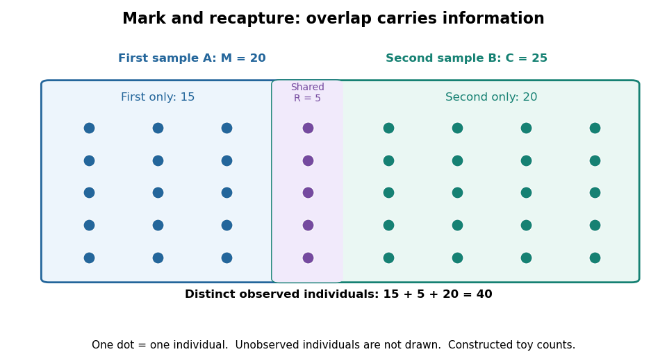
Forty distinct observed individuals: fifteen in the first sample only, five shared, and twenty in the second sample only
. **Details**.

The diagram shows only observed individuals. It does not draw an assumed population of one hundred. The capture-recapture model uses the overlap to infer how many individuals may have escaped both samples; its likelihood function shows why one estimator output cannot describe all that uncertainty.

Capture-recapture model

A capture-recapture model is a statistical model for repeated observations of identifiable individuals, including those missed on some occasions. A closed-population capture-recapture model estimates a fixed population cardinality; models allowing individuals to enter or leave can instead describe survival and recruitment. The sampling assumptions determine which likelihood function is appropriate.

For the two-sample closed-population capture-recapture model, condition on the sample sizes

M

and

C

. If the second sample selects

C

distinct individuals from

N

by simple random sampling, then the overlap

R

has the hypergeometric distribution:

P (R = r ∣ N, M, C) = \frac{( r M ) ( C - r N - M )}{( C N )}, max (0, M + C - N) \leq r \leq min (M, C) .

Here

r

is an integer and the probability mass function is zero outside these bounds. The binomial coefficients count choices of

r

marked and

C - r

unmarked individuals, divided by all equally likely size-

C

subsets. The hypergeometric distribution has expected value

E [R ∣ N, M, C] = \frac{MC}{N} .

(2)

Equating the observed overlap with this expected value gives the Lincoln-Petersen estimator. The underlying sampling without replacement, probability mass function, and expected value are developed in Raymond P. Guiteras, MIT 14.30 hypergeometric distribution handout, §§1–4 and 8.

For the toy counts

M = 20

C = 25

, and

R = 5

, hold the observations fixed and vary the unknown integer

N

. The likelihood function is

L (N) = \frac{( 5 20 ) ( 20 N - 20 )}{( 25 N )}, N = 40, 41, 42, \dots .

(3)

Values below forty cannot contain the observed set union. Exact comparison of consecutive likelihoods gives two tied maximum-likelihood estimates,

N = 99

and

N = 100

. The Lincoln-Petersen estimator returns

100

; the Chapman estimator returns

90

and is a different rule for estimation.

Figure 1.
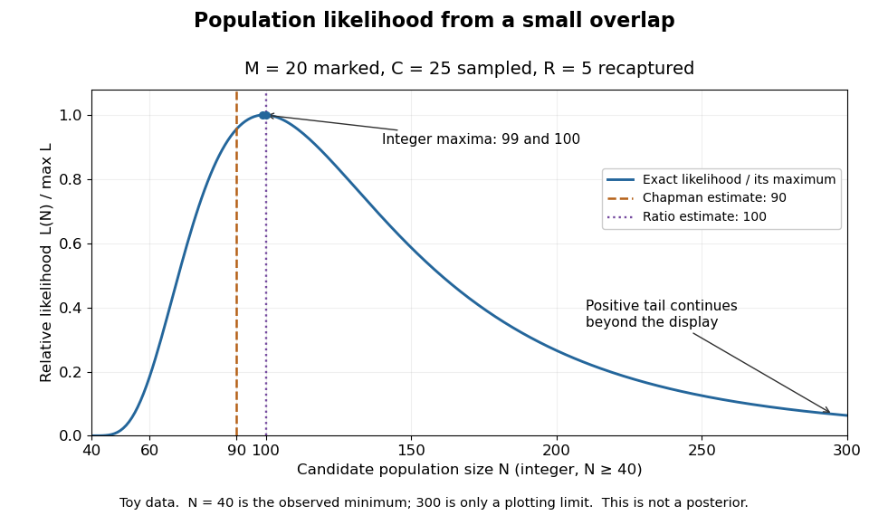
Relative likelihood for the toy overlap: integer maxima at 99 and 100, ratio estimate 100, and Chapman estimate 90
. **Details**.

The vertical scale is

L (N) / max_{n \geq 40} L (n)

. This relative likelihood compares how well candidate statistical parameters explain the same observations; it is not a posterior probability. The displayed range

40 \leq N \leq 300

is only a plotting window. The likelihood function remains positive for every integer

N \geq 40

and tends to zero as

N

increases, so the curve has a continuing right tail. The data do not justify truncating statistical inference at three hundred. The conditional hypergeometric distribution formulation also appears in Louis-Paul Rivest and Mamadou Yauck, Small Sample Estimators for Two-way Capture Recapture Experiments, §3, equation (5).

Zero recaptures require care. With

R = 0

and positive

M, C

, the Lincoln-Petersen estimator has no finite ratio, but the capture-recapture model still gives a valid likelihood function:

L_{0} (N) = \frac{( C N - M )}{( C N )}, N \geq M + C .

(4)

This likelihood function increases toward one as

N

grows, so there is no finite maximum-likelihood estimate. For the same sample sizes twenty and twenty-five with zero overlap, forty-five distinct individuals would be observed. Lack of overlap supplies a lower bound but very weak information about large population cardinalities.

In more elaborate capture-recapture models, a first-recapture array

m_{ij}

counts individuals released at occasion

i

and next observed at

j

. A probability of survival

ϕ_{j}

and a probability of detection

P_{j + 1}

contribute a no-observation continuation factor

ϕ_{j} (1 - P_{j + 1})

. The resulting likelihood function depends on both survival and detection; these probabilities need not be separately identifiable at the last observation interval. Missing-count EM for capture-recapture describes one way to fit such a model, and identifiability remains a separate issue from computing an estimator output.

Closed-population capture-recapture model ( $N = constant$ )

A closed-population capture-recapture model assumes the same individuals remain throughout the observations: no births, deaths, immigration, or emigration. Its elementary two-sample version additionally requires retained, correctly recognized marks and a second sample chosen by simple random sampling independently of first-sample membership. Mixing and unchanged capture behavior help make this plausible. Equal individual capture probabilities alone do not guarantee that every size-

C

subset is equally likely; that stronger sampling assumption gives the hypergeometric distribution. See Barker, §§1.1.1 and 1.1.3: closure, marks, and catchability assumptions.

Unequal catchability, mark loss, and population change can invalidate this capture-recapture model. For example, if especially catchable individuals appear repeatedly, overlap can be inflated and the Lincoln-Petersen estimator can underestimate population cardinality. Lost marks can decrease recorded overlap and increase the same ratio estimator, all else equal. Two samples alone cannot establish that the sampling assumptions hold.

Lincoln-Petersen estimator ( $N_{LP} = MC / R$ )

The Lincoln-Petersen estimator is the ratio estimator obtained by matching the observed overlap to its hypergeometric expected value. It is defined when

R > 0

. To distinguish that ratio from the exact integer maximization, consecutive positive likelihoods satisfy

\frac{L ( N + 1 )}{L ( N )} = \frac{( N + 1 - M ) ( N + 1 - C )}{( N + 1 ) ( N + 1 - M - C + R )} .

This comparison is valid for

N \geq M + C - R

. For the toy counts, the numerator minus the denominator is

500 - 5 (N + 1)

. Thus the likelihood function increases up to ninety-nine, ties at ninety-nine and one hundred, then decreases for every larger integer. This independently establishes the global maximum-likelihood estimates, beyond the plotting window. The adjacent-ratio method is given in Guiteras, §8.

Chapman estimator ( $N_{Ch} = \frac{( M + 1 ) ( C + 1 )}{R + 1} - 1$ )

The Chapman estimator is a correction intended to reduce the small-sample bias of the Lincoln-Petersen estimator. Under the fixed-size hypergeometric sampling assumptions it is exactly an unbiased estimator when

M + C \geq N

; it can have nonzero bias otherwise. This qualification and the formula are stated in Barker, §1.1.1, equation (1.3), citing Chapman's work through Seber. For the toy observations,

N_{Ch} = \frac{( 20 + 1 ) ( 25 + 1 )}{5 + 1} - 1 = \frac{546}{6} - 1 = 90.

It is an alternative estimator, not a maximum-likelihood estimate for this capture-recapture model. The Chapman estimator remains finite when

R = 0

, but a finite output does not supply the missing overlap information or repair unequal catchability, lost marks, or population change.

Missing-count EM for capture-recapture ( $E [n_{ij} ∣ m, ϕ, P] = N_{i} w_{ij} / C_{i}$ )

Let

N_{i} = R_{i} - \sum_{s = i + 1}^{J} m_{i s}

count individuals never recaptured after release

i

. Partition them into death-interval counts

n_{ij}

and terminal survivors

n_{i J}

. Their unnormalized weights are

w_{ij} = (1 - ϕ_{j}) \prod_{ℓ = i}^{j - 1} ϕ_{ℓ} (1 - P_{ℓ + 1})

for

j < J

, and

w_{i J} = \prod_{ℓ = i}^{J - 1} ϕ_{ℓ} (1 - P_{ℓ + 1})

. Conditional counts are multinomial with normalizer

C_{i} = \sum_{j = i}^{J} w_{ij}

. The EM algorithm replaces all missing counts by the displayed conditional expectations, then maximizes the resulting complete-data log likelihood. Survival and detection updates are expected successes divided by expected opportunities. A flat observed-likelihood ridge remains nonidentifiable even if each conditional complete-data maximization is explicit.

Nonlinear regression

Nonlinear regression fits a conditional mean whose dependence on its parameters is nonlinear. In a normal distribution observation model, the likelihood is based on residuals

y_{i} - m (x_{i}, θ)

. Nonlinearity can create parameter trade-offs, asymmetric uncertainty and several posterior regions, so prior predictive checks and Markov chain Monte Carlo convergence diagnostics can be especially useful.

Outlier

An outlier is an observation unusually far from the behavior expected under a statistical model. A large regression residual can identify a candidate, but data validation, regression leverage, and the possibility of model misspecification should be examined before excluding it. An outlier need not be an influential observation.

Regression to the mean

An unusually extreme noisy observation tends to be followed by a less extreme observation even without intervention. Selecting locations for an intervention because they had high prior event counts can therefore bias a simple before-and-after comparison toward an apparent reduction. The effect follows from conditioning on an extreme value with a transient random component, rather than from a causal treatment effect.

Response variable ( $Y$ )

A response variable is the outcome whose variation is described by a statistical model or whose change is compared across treatments. Its unit, measurement procedure and observation time must be specified. An outcome consisting of a feature count is one response per sketch, not one independent experimental response per feature.

Scientific control

A scientific control supplies a comparison or procedure that distinguishes an intended effect from other influences on an experiment or observational measurement. Negative controls should show no target effect; positive controls should show a known effect. A negative control outcome applies this logic to an outcome that the exposure cannot causally affect.

Design of experiments

Design of experiments chooses experimental units, treatments, replication, blocks in experimental design and randomization so that scientifically useful treatment contrasts can be estimated with meaningful standard errors. Allocation determines which measurements supply independent treatment information.

Optimal experimental design

Optimal experimental design chooses observation locations and allocations to optimize a specified criterion for a specified statistical model. Criteria can control the determinant of an estimator's covariance matrix or its worst prediction variance. Optimality depends on the model and the permitted design class, including whether allocations are integer or approximate.

General equivalence theorem for optimal design

For continuous regressors spanning a

p

-dimensional space on a compact design region, and approximate designs with nonsingular information matrix of an experimental design, the following are equivalent: D-optimal design, G-optimal design, and

sup_{x} d (x, ξ) = p

. A D-optimal design has nonpositive directional derivatives

d (x, ξ) - p

. Conversely, if every such derivative is nonpositive, concavity of

lo g det

bounds every competing information matrix by the tangent at

M (ξ)

, proving D-optimality. The sensitivity average is

p

, and a D-optimal design exists by compactness of the information-matrix set and the spanning assumption; hence the optimal G-value is

p

. Sensitivity equals

p

at every support point of an optimal design. The equivalence concerns approximate allocations; integer restrictions can change exact-design optima.

G-optimal design ( $min_{ξ} sup_{x} d (x, ξ)$ )

A G-optimal design minimizes the maximum design sensitivity function over the full design region. Thus it minimizes the worst variance of a fitted regression mean, excluding the separate noise variance of a new observation. The sensitivity average is

p

, so its supremum is at least

p

D-optimal design ( $max_{ξ} det M (ξ)$ )

A D-optimal design maximizes the determinant of the information matrix of an experimental design, equivalently minimizing the determinant of the covariance matrix of a fixed-size least-squares estimator. It minimizes the volume of a fixed-level confidence ellipsoid for the model coefficients under the usual Gaussian model.

Approximate experimental design ( $ξ = \sum_{i} w_{i} δ_{x_{i}}$ )

An approximate design is a probability measure on the design region, with weight

w_{i}

specifying a proportion of observations at

x_{i}

. For

N

independent observations and common error variance

σ^{2}

, a linear regression with vector

f (x)

has normalized information matrix of an experimental design

M (ξ) = \int f (x) f (x)^{T} d ξ (x)

; its least-squares estimator has covariance

σ^{2} M (ξ)^{- 1} / N

when the allocations realize these proportions. Exact designs restrict

N w_{i}

to integers.

Information matrix of an experimental design ( $M (ξ) = \int f (x) f (x)^{T} d ξ (x)$ )

The normalized information matrix for a homoscedastic linear regression model is the average outer product of its regressor vector. It is positive-definite precisely when the supported regressors span the parameter space. The full Fisher information matrix under normal errors is

NM (ξ) / σ^{2}

Design sensitivity function ( $d (x, ξ) = f (x)^{T} M (ξ)^{- 1} f (x)$ )

The sensitivity function is the normalized variance of a fitted regression mean. Its average under the design is the number

p

of model coefficients, since

\int d d ξ = tr (M^{- 1} M) = p

. The directional derivative of

lo g det M

towards a point mass at

x

d (x, ξ) - p

Latin square

A Latin square of order

q

is a

q \times q

array of

q

symbols, each occurring once in each row and column. Used as a row-column design, its symbols label treatments. Centered treatment indicators are orthogonal to both row and column indicators, because every row-treatment and column-treatment pair occurs once. This balance separates additive effects from two nuisance directions.

Analysis of variance for a Latin square

For one response per cell in an order-

q

Latin square, fit an intercept and additive row, column and treatment effects with sum-to-zero constraints. Each factor contributes

q - 1

statistical degrees of freedom; the residual has

q^{2} - 1 - 3 (q - 1) = (q - 1) (q - 2)

. The centered factor spaces are mutually orthogonal, so sequential sums of squares do not depend on fitting order. With an additional orthogonal symbol factor from a Graeco-Latin square, residual statistical degrees of freedom become

(q - 1) (q - 3)

. Exact F-tests require independent equal-variance normal errors; unmodeled interactions can invalidate the error term.

Mutually orthogonal Latin squares

Latin squares on the same array are mutually orthogonal when every ordered pair of symbols from any two squares occurs exactly once on superposition. Pairwise balance makes the centered symbol-indicator spaces orthogonal in an additive linear regression model.

Graeco-Latin square

A Graeco-Latin square is the superposition of two orthogonal Latin squares of the same order. Each symbol of either square occurs once per row and column, and every cross-square pair occurs once. It permits four mutually orthogonal additive factor spaces: rows, columns, and the two symbol factors.

Contrast (statistics)

A contrast is a linear combination

\sum_{i} c_{i} μ_{i}

of group means with

\sum_{i} c_{i} = 0

. It compares responses without depending on a common additive level. Treatment contrasts and factorial contrasts specify comparisons in a design of experiments.

Response surface methodology

Response surface methodology fits local regression approximations to a quantitative response as experimental settings change. A first-order model estimates a local gradient; augmenting the design permits quadratic regression, curvature assessment and local optimization. Extrapolating a fitted surface outside the experimentally supported region requires caution.

Center-point curvature contrast ( $γ = \overset{ˉ}{Y}_{F} - \overset{ˉ}{Y}_{0}$ )

In a two-factor design with four corner observations and

n_{0}

independent center replicates, the difference between the corner mean and center mean has variance

σ^{2} (1/4 + 1/ n_{0})

. Under a full quadratic regression surface it estimates

β_{11} + β_{22}

; the linear and interaction terms average to zero at the corners. With

n_{0} \geq 2

, the center pure error estimate makes its squared standardized contrast an

F_{1, n_{0} - 1}

test under a first-order mean model. Zero contrast does not exclude curvature, since the two squared-term coefficients may cancel.

Steepest ascent in response surface methodology ( $d = b /∥ b ∥$ )

For a fitted local first-order response

m (x) = β_{0} + b^{T} x

, the unit direction maximizing its directional derivative in coded Euclidean distance is

d = b /∥ b ∥

, by the Cauchy-Schwarz inequality. Run sequential feasible settings

x_{0} + h d

, increase

h

while measured response improves, and refit near promising settings. Physical increments are

h_{j} h d_{j}

, so coded and unscaled physical gradients need not give the same experimental path. A near-zero gradient calls for further modeling rather than division by zero.

Coded experimental variable ( $x_{j} = (ξ_{j} - c_{j}) / h_{j}$ )

A coded experimental variable rescales a physical setting

ξ_{j}

around its center

c_{j}

, dividing by a chosen positive half-range

h_{j}

. The endpoints

c_{j} \pm h_{j}

become

\pm 1

, giving dimensionless factorial design coordinates. The choice of scale affects the metric used for steepest ascent in response surface methodology.

Rotatable design

A design for a specified polynomial model is rotatable when the variance of a fitted regression mean depends on a setting only through its distance from the centre. For a full

2^{d}

factorial portion plus symmetric axial points in a central composite design, fourth-order rotational symmetry requires

\sum x_{i}^{4} = 3 \sum x_{i}^{2} x_{j}^{2}

. These sums are

2^{d} + 2 α^{4}

and

2^{d}

, giving

α = (2^{d})^{1/4}

. Sign symmetry removes odd moments and equal second moments complete the required moment symmetry for a full quadratic model.

Central composite design

A central composite design augments a factorial portion with axial points

\pm α e_{j}

and replicated centre points. It supports a full quadratic response model: intercept, linear terms, cross-products and squared coordinates. Centre-point replication estimates pure error. Choosing the axial distance appropriately gives a rotatable design.

Split-plot design

A split-plot design randomizes one factor to whole plots and another to subplots within each whole plot. Whole-plot treatment effects and subplot treatment effects therefore use different error ANOVA strata. Whole plots provide replication for the first factor; their subplots do not supply extra independent whole-plot replication. Within-whole-plot comparisons can remove a shared additive whole-plot variance component.

Factorial design

A factorial design includes every combination of specified factor levels. Balanced replication permits separate estimation of marginal effects and interaction terms. The factor allocation, not the number of subsamples, determines the appropriate error term for each effect.

Main effect

A main effect compares the mean response at different levels of one factor after averaging over the other factors according to the design. With sign coding, its two-level difference is twice the singleton factorial contrast coefficient. In a fractional factorial design, that coefficient can include aliased higher-order effects.

Factorial contrast ( $χ_{A} (x) = \prod_{j \in A} x_{j}$ )

In a two-level factorial design, a factor subset defines a sign column. The coefficient of this column is its response contrast divided by the number of runs when the columns are orthogonal. A singleton describes a main effect and a pair describes a two-factor interaction. On the full cube, distinct columns have zero inner product: summing over any coordinate in their symmetric difference cancels the terms.

Fractional factorial design

A fractional factorial design uses a selected subset of the full factor-level combinations. In a regular two-level fraction, encode levels by signs and impose

k

independent equations

\prod_{j \in G_{i}} x_{j} = s_{i}

. Independence of the generator incidence vectors over

F_{2}

leaves

2^{m - k}

runs. Reduced run count creates aliasing in a fractional factorial design, which must be evaluated against the effects scientifically required.

Resolution of a fractional factorial design ( $R = min_{G \in H ∖ {I}} ∣ G ∣$ )

The resolution of a regular fraction is the shortest nonidentity word in its defining contrast subgroup. Two effects alias only when their word product belongs to that subgroup. Thus resolution VI separates all main effects and two-factor interactions from one another and from three-factor interactions, though some three-factor interactions alias in complementary pairs.

Defining contrast subgroup ( $H = ⟨ G_{1}, \dots, G_{k} ⟩$ )

Factor subsets multiply by symmetric difference; their sign columns multiply pointwise. The subgroup generated by independent defining words has

2^{k}

elements. On a selected fractional factorial design, every word in this subgroup is constant, with sign determined by the chosen generator signs. The cosets classify identical or opposite contrast columns.

Aliasing in a fractional factorial design ( $χ_{A G} = s_{G} χ_{A}$ )

Two factorial contrasts are aliased if their columns are proportional on the selected fractional factorial design. A word

G

that has fixed sign

s_{G}

gives

χ_{A G} = s_{G} χ_{A}

. Conversely, averaging a character over the fraction vanishes unless its word belongs to the defining contrast subgroup, so every alias class is exactly a subgroup coset. In a half fraction each class has two distinct words; their separate coefficients cannot be identified without assumptions or additional runs.

Crossover design

A crossover design assigns each subject a sequence of treatments in successive periods. Subject blocking can reduce between-subject variation; balanced sequences can separate treatment from period effects. A carryover effect or irreversible change can invalidate a simple within-subject comparison.

Carryover effect

A carryover effect is an effect of a previous treatment on a later response. Balanced transitions help prevent a treatment from being preceded disproportionately by one particular alternative, but do not ensure that carryover effects vanish or are separately identifiable in every model.

Completely randomized design