Bayes factor ($B_{01}$)

A Bayes factor measures how data change the relative support for two specified statistical models. Write $m_j(D)=p(D\mid H_j)$ for their Bayesian model evidence and define the direction explicitly:For positive finite $m_0(D),m_1(D)$, a value above one favors $H_1$ over $H_0$; a value below one favors $H_0$ over $H_1$. Reversing the comparison gives $B_{01}={\mathrm{BF}}_{01}=1/{\mathrm{BF}}_{10}$, the opposite direction used in some formulas below.

For mutually exclusive, exhaustive $H_0,H_1$ with positive prior probabilities, divide their two Bayes' theorem formulas. Their common data normalizer cancels, leavingThe Bayes factor therefore multiplies prior odds into posterior odds. It is evidence conditional on the specified statistical models and their within-model prior distributions; it is not $\mathbb{P}(H_1\mid D)$. Model prior probabilities supply a separate input.^[ref]

For an original stipulated example, consider ten independent and identically distributed Bernoulli trials, with heads as success. Compare $H_0:p=0.4$ with $H_1:p=0.7$, both fixed before seeing the data. Take $D$ to be one particular ordered sequence containing eight heads and two tails. The likelihood function under either point model is $p^8(1-p{)}^2$, soIf $\mathbb{P}(H_1)=0.1$, the prior odds for $H_1$ against $H_0$ are $1/9$. Hence the posterior odds are $21.9909706/9\approx 2.4434412$, andEqual model prior probabilities would instead give ${\mathrm{BF}}_{10}/(1+{\mathrm{BF}}_{10})\approx 0.956505$. The same Bayes factor can thus accompany different posterior probabilities. These statements condition on the two-model comparison; they do not establish that either statistical model describes a real coin.

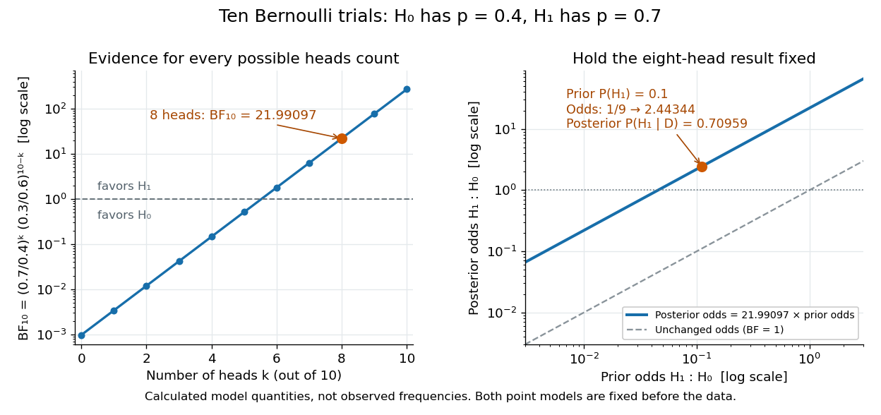
Using the heads count $K=8$ instead of the ordered sequence changes the sample space. The binomial distribution assigns it mass $\left(\genfrac{}{}{0ex}{}{10}{8}\right)p^8(1-p{)}^2$. The same binomial coefficient multiplies both models' Bayesian model evidence and cancels in their Bayes factor. Mixing an ordered-sequence numerator with a count denominator would introduce an erroneous factor of $45$.

Fix the candidate statistical models, their parameter prior distributions, and model prior probabilities before using the current data for this update. The Bayes factor is useful because it separates evidence from model prior odds, but it still depends on the parameter prior distributions. An improper prior has an arbitrary multiplicative normalization: multiplying its kernel by $c$ multiplies its formal marginal likelihood by $c$, even if the within-model posterior distribution is normalizable. Without a separately justified convention, the ordinary Bayes factor is then undefined up to arbitrary constants.^[ref]

For a binomial distribution count, compare a point null $\theta =1/2$ with the uniform alternative prior distribution on $(0,1)$. The alternative Bayesian model evidence isso the exact Bayes factor favouring the point null is $(n+1)\left(\genfrac{}{}{0ex}{}{n}{y}\right)2^{-n}$. With standardized deviation $z=2(y-n/2)/\sqrt{n}$, the local normal distribution approximation is $B_{01}\approx \sqrt{2n/\pi }{e}^{-z^2/2}$. At fixed $z$ the frequentist p-value remains approximately constant, while the factor grows like $\sqrt{n}$. This demonstrates the prior-width mechanism behind the Jeffreys-Lindley paradox for a Gaussian point null in a discrete sampling model.

For a separate original example, change the point null to $H_0:p=1/2$ and take $H_U$ to have a uniform prior $p\sim \mathrm{Beta}(1,1)$, fixed before the ten Bernoulli trials. Here $p$ is drawn once under $H_U$ and shared by all ten trials: they are independent conditional on $p$. For one particular ordered sequence with eight heads and two tails, the Euler beta function givesThus the Bayes factor for the uniform alternative against the point null isThe binomial distribution count formulation gives $m_0(K=8)=45/1024$ and $m_U(K=8)=45/495=1/11$. Their ratio is again $1024/495$; these count masses must not be combined with the ordered-sequence masses above. The general $B_{01}$ formula at the start of this article puts the point null in the numerator, so it equals $B_{0U}$ here.

In contrast, maximum likelihood estimation gives $\hat{p}=0.8$: differentiating the log-likelihood yields $8/p-2/(1-p)=0$, and the endpoints have zero likelihood. Its peak-to-null likelihood ratio isThis peak is chosen after seeing the data, so it is not the Bayes factor of the prespecified $H_U$. The Bayesian model evidence for $H_U$ averages $L(p)$ over its entire uniform prior; it is smaller than the peak. It is also smaller than $L(0.7)=0.7^{8}0.3^2\approx 0.00518832$. Against the same $p=0.5$ null, a point alternative fixed at $p=0.7$ would give a Bayes factor about $5.31284$, greater than $2.06869$. An integrated alternative need not outperform a point alternative.

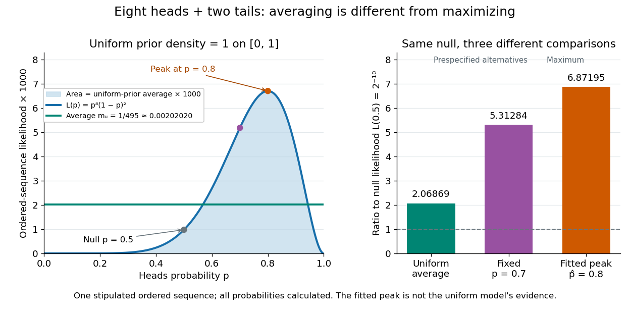
For a general proper beta distribution prior distribution $\mathrm{Beta}(a,b)$ with $a,b>0$, the same ordered-sequence marginal likelihood is $B(8+a,2+b)/B(a,b)$. This follows by substituting the normalized prior density into the integral, and shows exactly where the parameter prior distribution changes the Bayes factor. Holding the parameter prior distributions fixed while changing model prior odds leaves that Bayes factor unchanged.

A Gaussian practical-null mixture compares a narrow centered normal distribution prior with a wider centered normal distribution prior. Neither component is a point mass. With observed mean $y\mid \beta \sim N(\beta ,1/n)$ and prior precisions $q_0>q_1>0$, its model predictive variances are $V_i=1/n+1/q_i$, and the Bayes factor isThe overall posterior density is a Bayesian model averaging mixture with component means $ny/(n+q_i)$. A wide-prior penalty can favor the practical null near zero; its dominance depends quantitatively on both prior scales and the observation, not merely on the observation being of order $n^{-1/2}$.

For suitable nested models whose common nuisance parameters have matching priors, the Savage-Dickey density ratio expresses a Bayes factor as posterior density divided by prior density at the nested parameter value.