 Polynomial identity testing over a finite field

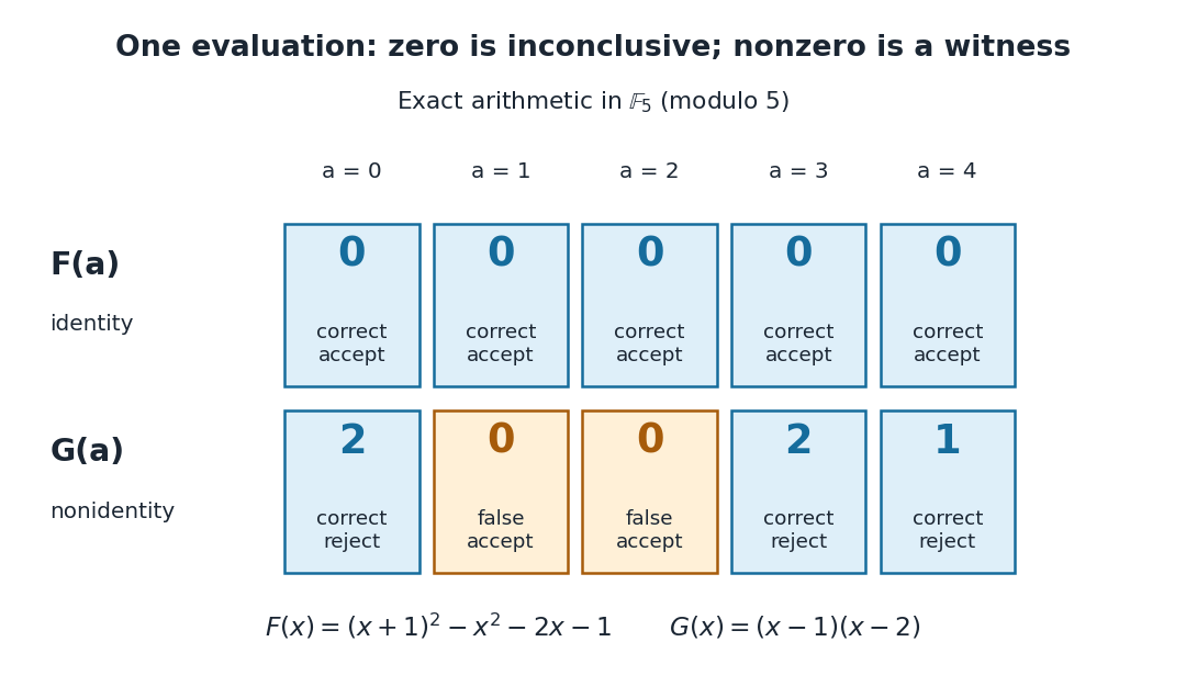
Work in the finite field ${\mathbb{F}}_5=\{0,1,2,3,4\}$, using modular arithmetic modulo five. Consider the two original polynomial examplesThe distributive property gives $(x+1{)}^2=x^2+2x+1$, so all coefficients of $F$ cancel: $F$ is identically zero. In contrast, $G=x^2-3x+2=x^2+2x+2$ in this finite field, with nonzero leading coefficient. Its roots of a polynomial are exactly one and two: a product in a field is zero only if a factor is zero.

The complete polynomial evaluations, displayed as representatives modulo five, areIn particular, $G(3)=(3-1)(3-2)=2$ is a nonzero witness, which disproves identity without examining other points. At one or two, a zero value fails to reveal that $G$ is nonzero. A random variable $a$ with a uniform distribution on a finite set ${\mathbb{F}}_5$ hits those two polynomial roots with probability $2/5$.

A crucial limit appears with $H(x)=x^5-x$. Its coefficients make it a nonzero polynomial of polynomial degree five in ${\mathbb{F}}_5[x]$, yet direct polynomial evaluation gives zero at all five field elements: the values before reduction are $0,0,30,240,1020$, all divisible by five. Thus $H$ induces the same polynomial function as the zero polynomial. Any number of trials restricted to ${\mathbb{F}}_5$ will falsely accept this identity. This is compatible with the Schwartz-Zippel lemma: the ratio of polynomial degree to sampling-set size is $5/5=1$, which gives no useful guarantee.

When a polynomial's representation permits polynomial evaluation over a larger field extension, a larger sampling set can restore the useful degree ratio. Access only to the induced polynomial function on the original finite field cannot distinguish $H$ from zero.^[ref]