Temporal optical coherence
ID: temporal-optical-coherence

Temporal optical coherence compares a field at one position with a delayed copy. In a Michelson interferometer, unequal round-trip lengths supply this delay. Even a source with rapidly changing wave phase can give high interferometric visibility close to zero delay, because both arms then deliver nearly the same source history. A source narrowed in optical spectrum generally retains correlation over larger delays; a single width does not describe sources with several separated lines. [ref]
https://ocw.mit.edu/courses/2-71-optics-spring-2009/bebe78c6a2ae2603a0d1a3ea85e0b4ca_MIT2_71S09_lec22.pdf. MIT 2.71/2.710, lecture 22, slides 2–5: temporal and spatial coherence
.For a stationary scalar field, choose the carrier convention , with frequency in cycles per second. Let be its spectral density per unit frequency, with . Its normalized field correlation is the Fourier transformThe optical spectrum weights the rotating contributions; a broad spread of frequencies allows them to cancel at short delays. This is the stationary field correlation–spectrum relation. The relevant spectrum is that of the optical field in the detected mode, rather than the low-frequency fluctuations of a detector's light intensity. [ref]
https://www.rp-photonics.com/optical_spectrum.html. Rüdiger Paschotta, RP Photonics Encyclopedia, Optical Spectrum: optical field spectrum and temporal coherence
.Here are two stipulated line profiles, each centered at with full width at half maximum . Write and use normalized profiles on the whole detuning line:The first is a Lorentzian, mathematically a Cauchy distribution; the second is a Gaussian function. Taking their Fourier transforms gives, with the carrier factor omitted from the magnitudes,These are calculated model results, not measured line profiles. The detuning approximation treats the narrow line as extending to arbitrarily large positive and negative ; for optical applications require . Exact spectra of the complex positive-frequency field have no negative absolute frequencies. Changing to angular frequency replaces by ; it must not silently preserve the same numerical constant.
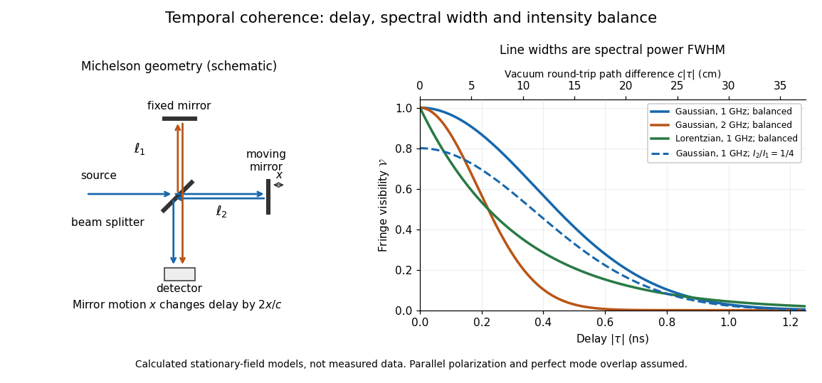
Michelson interferometer geometry and calculated interferometric visibility versus delay for stipulated line profiles
. Details. 
Equal detected single-arm light intensities give interferometric visibility equal to the correlation magnitude. Doubling the Gaussian full width at half maximum from to halves every fixed-contrast delay. At the model gives Gaussian interferometric visibility approximately at and at ; the Lorentzian gives . The dashed curve instead keeps the Gaussian correlation and changes to , multiplying all interferometric visibilities by . Its lower contrast at zero delay therefore comes entirely from intensity imbalance.
New to topics? Read the docs here!