
For a continuous random variable, the probability density integrates to the probability of an interval:Individual endpoints have zero probability, so strict or non-strict inequalities give the same answer.
With , integrating givesThe other two partial derivatives require . The origin condition fixes the remaining constant to zero. Hence the scalar potential isIts value at gives , so
A continuously differentiable conservative vector field has zero curl. HereThis vanishes everywhere if and only if . Since the field is smooth on the simply connected domain , zero curl is also sufficient; the explicit scalar potential in the next part confirms it.
A line integral uses , including the tangent vector. With , , the three components sum toConsequently
At each regular point, the gradientis normal to the level set and points towards increasing . The arrows in the contour plot above show this direction; their lengths have been normalized to keep the outer arrows legible. Near the origin they point outwards, as expected for a local minimum. Near , write ; the linear approximation is . Thus the arrows point away along the horizontal direction and towards the point along the vertical direction. The other two saddle points have the same behaviour after rotations through . All four stationary points have zero gradient, so no direction arrow is assigned at the points themselves.
The most useful guide to the contour plot is the common saddle value. Direct polynomial factorization givesThus the level set is exactly the three complete linesTheir intersections are the three saddle points, and they enclose the origin in an equilateral triangle. Near the local minimum, the level sets are nearly circles because the leading term is . For , a closed contour surrounds the origin, while three separate open branches lie outside the triangular barrier. At the saddle level these components meet at the saddle points; above it the central closed contour has opened into the three outer channels.
The identity in polar coordinatesshows the rotation symmetry through . It identifies the function as the Hénon-Heiles potential and helps organize all three channels in the original sketch below. The dashed straight lines are the saddle level; labels on the other contours give .
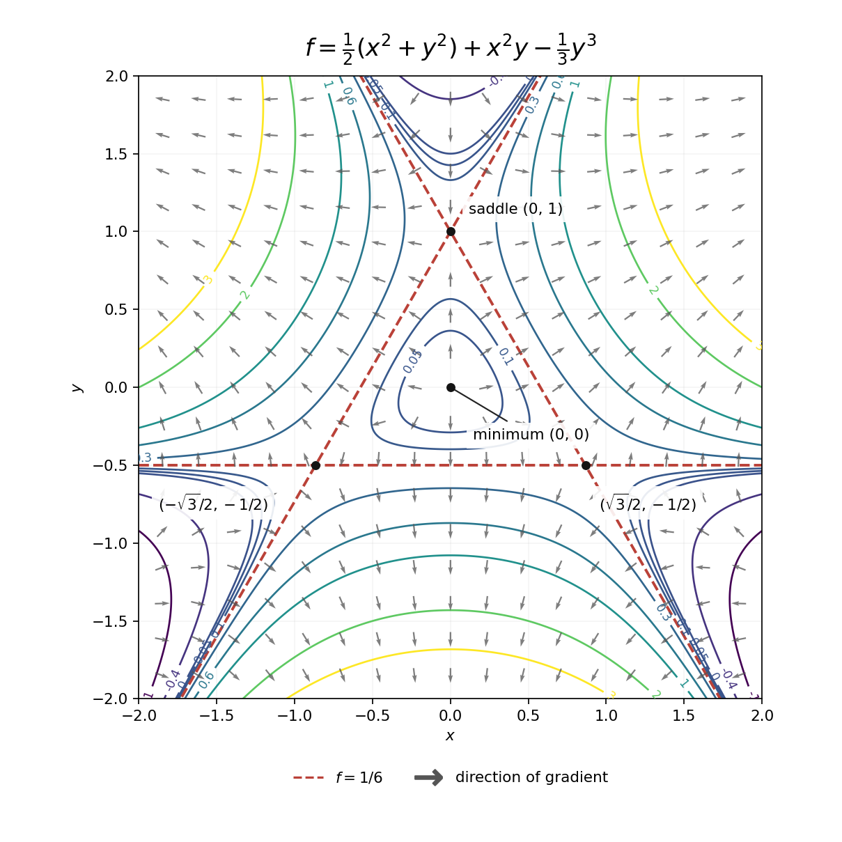
Contours and gradient directions of the Hénon-Heiles potential
. Details. 
The Hessian matrix isAt the origin it is the identity, so the origin is a strict local minimum. At it is , so this point is a saddle point. At either remaining stationary point,which again gives a saddle point. All three saddle points have eigenvalues and ; there are no local maxima.
There are unlisted articles, also show them or only show them.