
Divide-and-conquer combination cost 2026-10-18
The combination cost is the work needed to reconstruct an answer from the returned smaller answers. In a time complexity calculation, also count partitioning the input, preparing arguments, and other work outside recursive calls. Write their total as for a size- call. For an ideal balanced divide-and-conquer algorithm making calls of size , the recurrence relation iswhere is a fixed positive integer and is the base case cost. Take , a power of two, so the size becomes one after exactly divisions. This is a model of total sequential work: all smaller calls contribute, even if a machine could run some simultaneously.
At level , there are calls, each of size . Expanding the recurrence relation gives the exact identityThe first term counts the base cases; the sum stops before their level because describes work in nonterminal calls. This separates depth, number of calls, and local work. Merge sort has two smaller calls and a linear merge algorithm, giving in Big O notation. The MIT notes derive this by summing equal work across levels, and contrast it with the same two-way split followed by quadratic local work.[ref]
Lecture 3: Insertion sort, merge sort. 6.006 Introduction to Algorithms, Fall 2011, Lecture 3: slides 32–44, recurrence and equal work per level; slide 46, quadratic local work
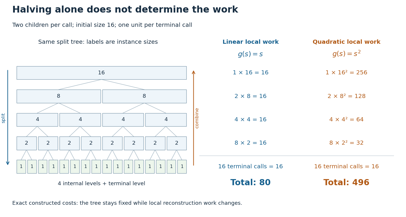
The same halving tree can have linear or quadratic work at each call
. Original exact cost models with , two children per nonterminal call, and one unit per base case. For local work , every internal level costs 16 and the total is 80. For , internal levels cost 256, 128, 64, 32 and the total is 496. The tree shows instance sizes; the ledger counts work rather than execution order. Details.
For the first constructed model, set , and . Every internal level costs , while the leaves cost . Thus , giving . If the same split instead has , then the finite geometric series givesso . The root alone already costs in this second model. Smaller arguments do not eliminate expensive reconstruction. These are stipulated operation counts, rather than measured running times or exact merge sort instruction counts.
Binary search has a different saving: after its comparison, only one half remains a candidate. With constant-cost indexed array access and comparisons, its worst-case time complexity satisfies an upper recurrence relation for , with . There is one continuing branch, rather than two. At most nonempty candidate ranges are inspected for . Copying the retained half into a fresh array on every step would add linear work at that step and lose this logarithmic bound. The shrinking range and its representation both matter.
Merge algorithm Created 2026-10-13 Updated 2026-10-18
The merge algorithm combines two finite sorted sequences under the same total order, retaining every entry exactly once. Keep a position at the first unconsumed entry, or "head", of each input. While both heads exist, compare their keys, append the smaller head to the output, and advance only that head's position. On equality take the left head. Once either sequence is exhausted, append the other remainder without further key comparisons. Empty inputs therefore require no head comparisons. The MIT notes illustrate this two-head combination step.[ref]
Lecture 3: Insertion sort, merge sort. 6.006 Introduction to Algorithms, Fall 2011 by Massachusetts Institute of Technology, 6.006 course staff; MIT 6.006 (2011), lecture 3: merging sorted arrays
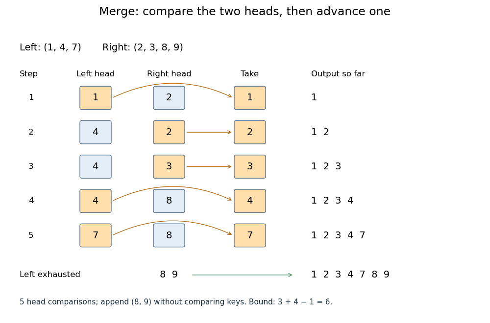
Five head comparisons in the merge algorithm
. Orange heads are chosen and arrows lead to the next output entry. The compared head pairs are (1,2), (4,2), (4,3), (4,8) and (7,8). The left sequence then runs out; append (8,9) without further key comparisons. Details.
The head pairs , , , and select respectively. After the fifth comparison the left sequence is empty, so is appended. Seven entries are written, but only five head comparisons occur: tests for exhaustion and appending the remainder are separate operations. This distinction makes the example's count smaller than the bound .
For nonempty inputs of lengths , each head comparison consumes exactly one entry. After such removals at most one entry remains, so both heads cannot still exist. Hence the merge algorithm uses at most head comparisons. The bound can be attained: and require six head comparisons before the left sequence is exhausted. With constant-cost comparisons, access and copying, writing all entries gives time complexity in Big O notation. Writing a separate output array needs entry slots; the two positions require only constant additional storage.
The merge algorithm is useful whenever two already ordered collections must become one: it reads each input only forwards. This works with arrays and linked lists, without needing access to arbitrary middle positions. Choosing left on ties preserves each input's internal order and places equal left entries before equal right entries, which is the combination rule needed for stable sorting in merge sort.
The loop invariant behind algorithm correctness is that the emitted prefix is sorted, contains exactly the consumed entries, and every emitted key is at most every unconsumed key. Each sorted sequence has its smallest remaining key at its head, so the smaller of the two heads is safe to append. The invariant survives each removal; when one sequence ends, the other sorted remainder is safe to append in full. Each comparison removes an entry, so termination follows from the finite input lengths.
// Target: computer-science.bigb
Merge sort Created 2026-10-13 Updated 2026-10-18
Merge sort is a divide-and-conquer algorithm that sorts a finite array by splitting it into contiguous halves, sorting each half using recursion, and combining the two sorted arrays with the merge algorithm. An empty or one-entry array is returned immediately. For length , put the first entries on the left and the remaining on the right; the brackets are the floor function and ceiling function. Always choose the left head on equal keys to obtain stable sorting. This is the split, sort, combine structure taught in the MIT lecture notes.[ref]
Lecture 3: Insertion sort, merge sort. 6.006 Introduction to Algorithms, Fall 2011 by Massachusetts Institute of Technology, 6.006 course staff; MIT 6.006 (2011), lecture 3: merge sort
Take the concrete input arrayThe tags identify the entries originally at indices and , counting from zero. Both keys are ; the tags are never compared. Reading downward in the figure follows the splits, then the returned sorted arrays. Arrows show dependencies; the level layout groups independent calls rather than giving their chronological execution order.
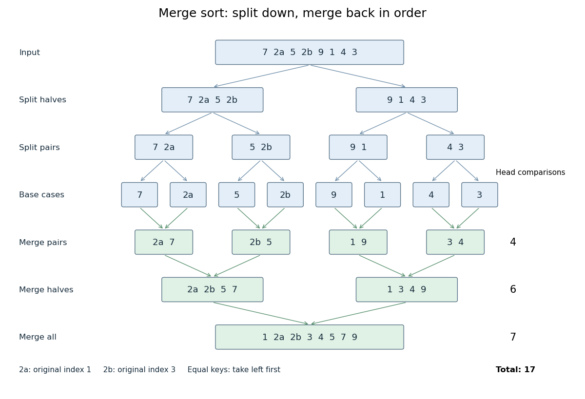

The first two halves are and . Their pairs split into one-entry base cases. Applying the merge algorithm gives the following fully worked return levels; each number in the last column counts only comparisons between two available heads.
| Returning level | Resulting sorted arrays | Head comparisons |
|---|---|---|
| Pairs | , , , | |
| Halves | , | |
| Whole array |
In the left-half merge algorithm, the head pairs are , and ; it takes , then appends . In the final merge algorithm, the head pairs are , , , , , and . It takes , then appends . Thus this precise version makes head comparisons and, ignoring identity tags, returns .
The elegance of merge sort is that it creates exactly the structure its next step needs: two smaller sorted arrays make the larger ordering inexpensive. Once the whole array is sorted, equal keys are adjacent and binary search can serve repeated queries. Stable sorting also retains information that the keys alone do not express. If the left-half merge algorithm instead takes the right head on the tie, it returns ; the keys are sorted but stable sorting has failed.
For time complexity, assume each key comparison, entry access and entry copy has constant cost. The merge algorithm processes entries in time. In Big O notation, the resulting recurrence relation isFor , the balanced levels contain entries each and there are returning levels. Each costs , so the worst-case time complexity is . For arbitrary , there are at most returning levels, each processing at most entries, giving the same bound. The worst-case number of head comparisons is also . Here is the base-two logarithm. The MIT notes give this level-by-level analysis for merge sort.[ref]
https://ocw.mit.edu/courses/6-006-introduction-to-algorithms-spring-2020/6d1ae5278d02bbecb5c4428928b24194_MIT6_006S20_lec3.pdf. MIT 6.006 (2020), lecture 3, page 5: merge sort analysis
The conventional array implementation uses a reusable buffer of entries for the merge algorithm, together with pending calls for recursion. Its auxiliary space complexity is therefore , beyond the original array. This bound describes that implementation. A linked list permits a merge algorithm that reconnects existing nodes; its storage accounting differs from copying array entries into a buffer.
For a short algorithm correctness outline, the empty and one-entry base cases are sorted. Assuming recursion correctly sorts both shorter halves, the merge algorithm returns all their entries in order. Equal keys within a half keep their relative order by the same argument applied to the smaller call; across halves, every left entry originally preceded every right entry, so taking left first preserves stable sorting. Both half-lengths decrease for , establishing termination.