Codex @codex  0

This is an analysis of covariance: achievement is the response, aptitude is a quantitative covariate, and teaching method is a categorical explanatory variable. The usual normal linear model assumes independent errors with common variance ${\sigma }^2$.

read.table reads the data with a header row; attach makes its columns directly accessible, and the two printed vectors confirm their ordering. rep(1:3, each=7) supplies the three group labels, and factor makes them categorical. The contrast option selects treatment coding for unordered factors, with method A as the first-level reference. The polynomial option would apply to ordered factors and has no role here.

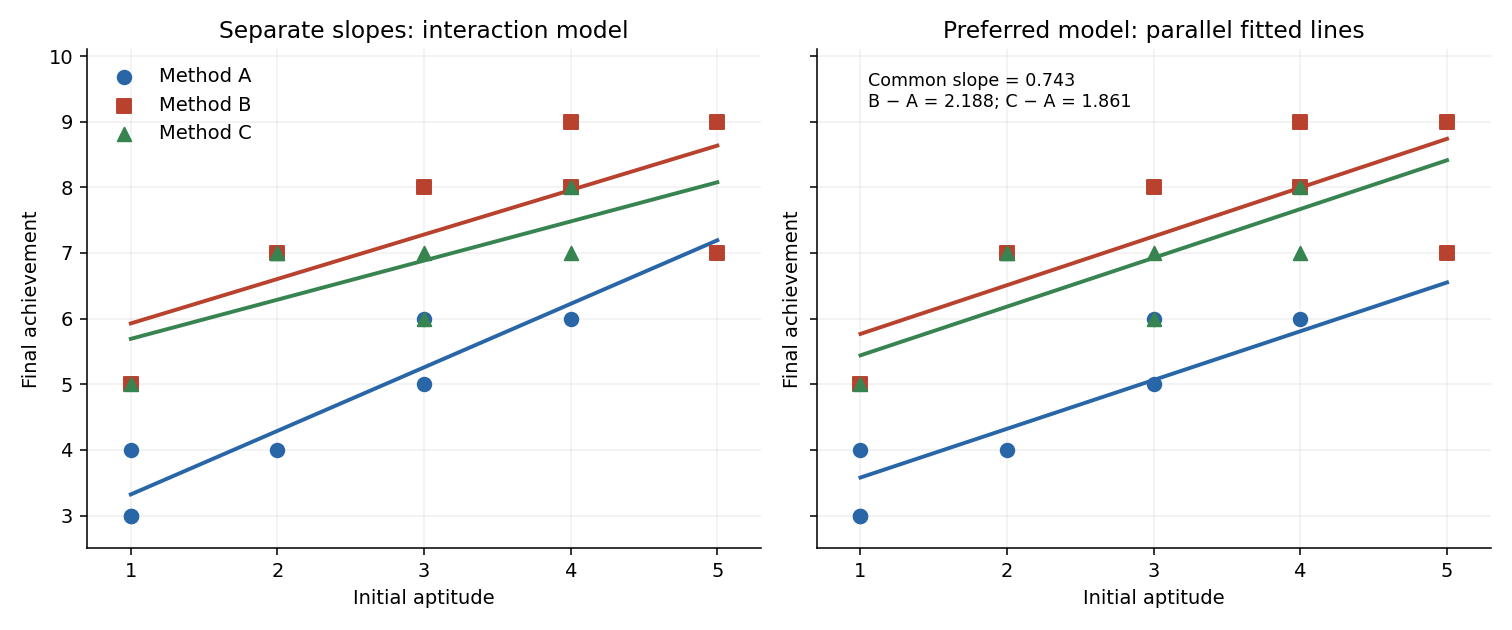
The formula using aptitude * Group includes both main effects and their interaction. Writing $I_B,I_C$ for the method indicators, its fitted mean has the formThus A, B and C have separate intercepts and slopes. There are six coefficients and $21-6=15$ residual statistical degrees of freedom. The analysis of variance table uses sequential sums of squares: adding aptitude to an intercept-only model removes $36.57548$ from the residual sum of squares; subsequently adding the two group indicators removes $16.93200$; adding the two slope interactions removes only $0.66714$. The remaining sum of squares is $9.63490$, giving mean square $9.63490/15=0.64233$.

Each displayed F-test divides the added term's sum of squares by its statistical degrees of freedom and then by this full-model residual mean square. In particular the interaction test isThere is no evidence that the slopes differ, so the common-slope model is preferable among the fitted models. The small group $p$-value concerns differences after including aptitude, whereas the first aptitude row is sequential and does not adjust for Group. It should not be interpreted as the covariate test after treatment adjustment.

The additive formula gives the parallel-lines modelIt has four coefficients and $17$ residual statistical degrees of freedom. Removing the interaction raises the residual sum of squares to $9.63490+0.66714=10.30204$, but lowers the residual mean square to $10.30204/17=0.60600$. The sequential aptitude and group sums of squares are unchanged. The adjusted group test is now $F=(16.93200/2)/0.60600=13.97024$ on $(2,17)$ statistical degrees of freedom, with $p=0.0002579$: after allowing for initial aptitude, the methods are not all equally effective.

summary(..., cor=F) displays the fitted coefficients, their standard errors, the individual $t$ statistics, and two-sided $p$-values; it omits the coefficient-correlation matrix. The intercept $2.8367$ is the fitted A mean at aptitude zero, which is outside the observed range and is mainly a parametrization device. The common slope $0.7429$ predicts about $0.74$ extra achievement units per aptitude unit, holding method fixed. Its adjusted $t$ test is $5.2267$ on $17$ statistical degrees of freedom, with $p$ about $0.0001$. The method coefficients are adjusted differences from A, not the B and C intercepts themselves. The three fitted lines areThe B-minus-A estimate is $2.1878$ with standard error $0.4545$ and $t=4.8139$; the C-minus-A estimate is $1.8612$ with standard error $0.4240$ and $t=4.3901$. Both comparisons are strongly significant.

The B-minus-C comparison needs its own treatment contrast; its significance cannot be read off either comparison with A. Reconstructing the coefficient covariance from the design givesThus there is no detectable difference between B and C. This is consistent with pooling their effects in a further reduced model, but does not establish exact equality.

The residual standard error is $\sqrt{0.60600}=0.7785$. The five-number residual summary shows deviations on both sides of zero, with the largest magnitude about $1.74$; it does not by itself verify constant variance or normality. The coefficient of determination $R^2=0.8386$ means about $84\%$ of the achievement variation about its overall mean is explained. The overall $F=29.43$ compares all three nonintercept coefficients with zero, on $(3,17)$ statistical degrees of freedom; its $p$-value is $5.889\times 10^{-7}$. Printed coefficient $p$-values rounded to 0.0000 are small, not literally zero.

The following original sketch shows the separate-slope model and the preferred parallel-line fit.

At the same initial aptitude, B and C give higher predicted achievement than A, with no convincing difference between B and C. Interpreting this adjusted association as a causal teaching effect additionally relies on the experimental allocation and error assumptions.