Coefficient of determination ($R^2$)

In an ordinary least squares regression with an intercept and a nonconstant response, $R^2=1-\mathrm{RSS}/{\sum }_i(Y_i-\overline{Y}{)}^2$. It measures the fitted proportion of sample variation relative to an intercept-only baseline. It increases when regressors are added, even if those regressors are unhelpful for prediction. A high value does not establish the assumptions of a normal linear model or rule out a systematic regression residual pattern.

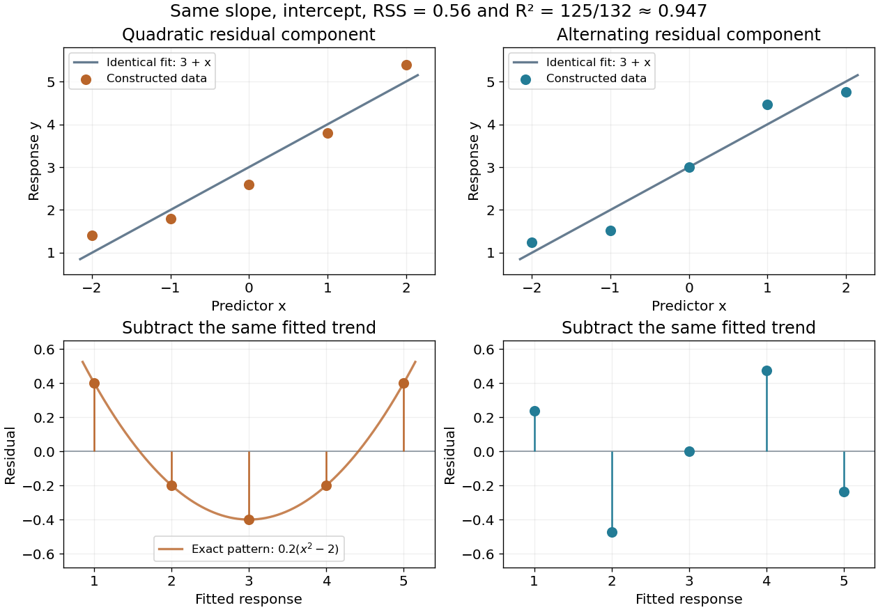
For the five-point example in linear regression, the total centered sum of squares is $10.8$ and the residual sum of squares is $0.8$, so $R^2=25/27\approx 0.926$. This summarizes the fitted reduction in squared error. It does not record the order or shape of the regression residuals, which are worth examining in a residual-versus-fitted plot.

Here is a fully constructed illustration. Use $x=(-2,-1,0,1,2)$ and the same fitted line $3+x$ for both datasets. Add respectively the residual vectorsBoth sum to zero, both have zero inner product with $x$, and both have squared norm $0.56$. Their ordinary least squares fit is therefore exactly the same line, with the same $R^2=10/(10+0.56)=125/132\approx 0.947$. But the first residual is $0.2(x^2-2)$, a systematic quadratic shape, while the second changes direction across the predictor values. These examples show directly which information the scalar $R^2$ discards; neither constructed pattern proves a random-error model.

In a normal linear model with an intercept, $n$ observations and $p$ independent mean coefficients, adjusted $R^2$ isIt compares the residual variance estimate with the unmodelled sample variance, adjusting the raw coefficient of determination for fitted dimension. It can be negative and is not guaranteed to increase when another regressor is added. In penalized regression a related convention uses the fit's effective degrees of freedom instead of $p$; the precise smoothing-software variance convention should be specified.